
Chapter 16
The Training Process
#hide
! [ -e /content ] && pip install -Uqq fastbook
import fastbook
fastbook.setup_book()#hide
from fastbook import *The Training Process
训练过程
You now know how to create state-of-the-art architectures for computer vision, natural language processing, tabular analysis, and collaborative filtering, and you know how to train them quickly. So we're done, right? Not quite yet. We still have to explore a little bit more the training process.
We explained in <<chapter_mnist_basics>> the basis of stochastic gradient descent: pass a mini-batch to the model, compare it to our target with the loss function, then compute the gradients of this loss function with regard to each weight before updating the weights with the formula:
new_weight = weight - lr * weight.gradWe implemented this from scratch in a training loop, and also saw that PyTorch provides a simple nn.SGD class that does this calculation for each parameter for us. In this chapter we will build some faster optimizers, using a flexible foundation. But that's not all we might want to change in the training process. For any tweak of the training loop, we will need a way to add some code to the basis of SGD. The fastai library has a system of callbacks to do this, and we will teach you all about it.
Let's start with standard SGD to get a baseline, then we will introduce the most commonly used optimizers.
你现在知道如何为计算机视觉、自然语言处理、表格分析和协同过滤创建最先进的架构,你也知道如何快速训练它们。那么我们就完成了,对吗?还没有。我们还得再探讨一下训练过程。
我们在<<chapter_mnist_basics>>中解释了随机梯度下降的基础:向模型传递一个小型批次,用损失函数与我们的目标进行比较,然后在用公式更新权重之前,计算这个损失函数对每个权重的梯度。
new_weight = weight - lr * weight.grad我们在训练循环中从头开始实现了这一点,同时也看到PyTorch提供了一个简单的nn.SGD类,可以为我们对每个参数进行这种计算。在本章中,我们将利用一个灵活的基础,构建一些更快的优化器。但这并不是我们在训练过程中可能想要改变的全部。对于训练循环的任何调整,我们都需要一种方法来为SGD的基础添加一些代码。fastai库有一个回调系统可以做到这一点,我们将教给你所有关于它的知识。
让我们从标准SGD开始,以获得一个基线,然后我们将介绍最常用的优化器。
Establishing a Baseline
确定基线
First, we'll create a baseline, using plain SGD, and compare it to fastai's default optimizer. We'll start by grabbing Imagenette with the same get_data we used in <<chapter_resnet>>:
首先,我们将创建一个基线,使用普通的SGD,并与fastai的默认优化器进行比较。我们先用<<chapter_resnet>>中使用的get_data抓取Imagenette。
#hide_input
def get_data(url, presize, resize):
    path = untar_data(url)
    return DataBlock(
        blocks=(ImageBlock, CategoryBlock), get_items=get_image_files,
        splitter=GrandparentSplitter(valid_name='val'),
        get_y=parent_label, item_tfms=Resize(presize),
        batch_tfms=[*aug_transforms(min_scale=0.5, size=resize),
                    Normalize.from_stats(*imagenet_stats)],
).dataloaders(path, bs=128)dls = get_data(URLs.IMAGENETTE_160, 160, 128)We'll create a ResNet-34 without pretraining, and pass along any arguments received:
我们将创建一个没有预训练的ResNet-34,并将收到的任何参数传递出去:
def get_learner(**kwargs):
    return vision_learner(dls, resnet34, pretrained=False,
                    metrics=accuracy, **kwargs).to_fp16()
Here's the default fastai optimizer, with the usual 3e-3 learning rate:
这是默认的fastai优化器,通常使用3e-3的学习率:
learn = get_learner()
learn.fit_one_cycle(3, 0.003)
Output
<IPython.core.display.HTML object>
| epoch | train_loss | valid_loss | accuracy | time |
|---|---|---|---|---|
| 0 | 2.571932 | 2.685040 | 0.322548 | 00:11 |
| 1 | 1.904674 | 1.852589 | 0.437452 | 00:11 |
| 2 | 1.586909 | 1.374908 | 0.594904 | 00:11 |
Now let's try plain SGD. We can pass opt_func (optimization function) to vision_learner to get fastai to use any optimizer:
现在我们来试试普通的SGD。我们可以把opt_func(优化函数)传给Vision_learner,让fastai使用任何优化器:
learn = get_learner(opt_func=SGD)The first thing to look at is lr_find:
首先要看的是lr_find:
learn.lr_find()Output
<IPython.core.display.HTML object>
(0.017378008365631102, 3.019951861915615e-07)
<Figure size 432x288 with 1 Axes>

It looks like we'll need to use a higher learning rate than we normally use:
看起来我们需要使用比我们通常使用的更高的学习率:
learn.fit_one_cycle(3, 0.03, moms=(0,0,0))Output
<IPython.core.display.HTML object>
| epoch | train_loss | valid_loss | accuracy | time |
|---|---|---|---|---|
| 0 | 2.969412 | 2.214596 | 0.242038 | 00:09 |
| 1 | 2.442730 | 1.845950 | 0.362548 | 00:09 |
| 2 | 2.157159 | 1.741143 | 0.408917 | 00:09 |
Because accelerating SGD with momentum is such a good idea, fastai does this by default in fit_one_cycle, so we turn it off with moms=(0,0,0). We'll be discussing momentum shortly.)
Clearly, plain SGD isn't training as fast as we'd like. So let's learn some tricks to get accelerated training!
因为用动量加速SGD是个好主意,fastai在fit_one_cycle中默认这样做,所以我们用moms=(0,0,0)关闭它。我们很快就会讨论动量问题)。
很明显,普通的SGD训练速度并不像我们希望的那样快。因此,让我们学习一些技巧来加速训练吧!
A Generic Optimizer
一个通用的优化器
To build up our accelerated SGD tricks, we'll need to start with a nice flexible optimizer foundation. No library prior to fastai provided such a foundation, but during fastai's development we realized that all the optimizer improvements we'd seen in the academic literature could be handled using optimizer callbacks. These are small pieces of code that we can compose, mix and match in an optimizer to build the optimizer step. They are called by fastai's lightweight Optimizer class. These are the definitions in Optimizer of the two key methods that we've been using in this book:
def zero_grad(self):
    for p,*_ in self.all_params():
        p.grad.detach_()
        p.grad.zero_()

def step(self):
    for p,pg,state,hyper in self.all_params():
        for cb in self.cbs:
            state = _update(state, cb(p, **{**state, **hyper}))
        self.state[p] = state
As we saw when training an MNIST model from scratch, zero_grad just loops through the parameters of the model and sets the gradients to zero. It also calls detach_, which removes any history of gradient computation, since it won't be needed after zero_grad.
为了建立我们的加速SGD技巧,我们需要从一个漂亮灵活的优化器基础开始。在fastai之前没有一个库提供这样的基础,但是在fastai的开发过程中,我们意识到所有我们在学术文献中看到的优化器改进都可以用优化器回调来处理。这些都是小块的代码,我们可以在优化器中进行组合、混合和匹配,以建立优化器step。它们被fastai的轻量级Optimizer类所调用。这些是我们在本书中一直使用的两个关键方法在Optimizer中的定义。
def zero_grad(self):
    for p,*_ in self.all_params():
        p.grad.detach_()
        p.grad.zero_()

def step(self):
    for p,pg,state,hyper in self.all_params():
        for cb in self.cbs:
            state = _update(state, cb(p, **{**state, **hyper}))
self.state[p] = state正如我们在从头开始训练MNIST模型时看到的那样,zero_grad只是在模型的参数中循环,并将梯度设置为零。它还调用detach_,删除任何梯度计算的历史,因为在zero_grad之后就不需要了。
The more interesting method is step, which loops through the callbacks (cbs) and calls them to update the parameters (the _update function just calls state.update if there's anything returned by cb). As you can see, Optimizer doesn't actually do any SGD steps itself. Let's see how we can add SGD to Optimizer.
Here's an optimizer callback that does a single SGD step, by multiplying -lr by the gradients and adding that to the parameter (when Tensor.add_ in PyTorch is passed two parameters, they are multiplied together before the addition):
更有趣的方法是step',它在回调(cbs')中循环,并调用它们来更新参数(_update函数只是在cb有任何返回时调用state.update)。正如你所看到的,Optimizer本身实际上并没有做任何SGD步骤。让我们看看如何将SGD添加到Optimizer中。
下面是一个优化器回调,通过将-lr乘以梯度,并将其添加到参数中,来完成一个SGD步骤(当PyTorch中的Tensor.add_被传递两个参数时,它们会在添加前被相乘):
def sgd_cb(p, lr, **kwargs): p.data.add_(-lr, p.grad.data)We can pass this to Optimizer using the cbs parameter; we'll need to use partial since Learner will call this function to create our optimizer later:
我们可以使用cbs参数将其传递给Optimizer;我们需要使用partial,因为Learner稍后将调用这个函数来创建我们的优化器:
opt_func = partial(Optimizer, cbs=[sgd_cb])Let's see if this trains:
让我们来看看这是否会产生影响:
learn = get_learner(opt_func=opt_func)
learn.fit(3, 0.03)
Output
<IPython.core.display.HTML object>
| epoch | train_loss | valid_loss | accuracy | time |
|---|---|---|---|---|
| 0 | 2.730918 | 2.009971 | 0.332739 | 00:09 |
| 1 | 2.204893 | 1.747202 | 0.441529 | 00:09 |
| 2 | 1.875621 | 1.684515 | 0.445350 | 00:09 |
It's working! So that's how we create SGD from scratch in fastai. Now let's see what "momentum" is.
它在工作! 因此,这就是我们如何在fastai中从头开始创建SGD。现在让我们看看什么是 "动量"。
Momentum
动量
As described in <<chapter_mnist_basics>>, SGD can be thought of as standing at the top of a mountain and working your way down by taking a step in the direction of the steepest slope at each point in time. But what if we have a ball rolling down the mountain? It won't, at each given point, exactly follow the direction of the gradient, as it will have momentum. A ball with more momentum (for instance, a heavier ball) will skip over little bumps and holes, and be more likely to get to the bottom of a bumpy mountain. A ping pong ball, on the other hand, will get stuck in every little crevice.
So how can we bring this idea over to SGD? We can use a moving average, instead of only the current gradient, to make our step:
weight.avg = beta * weight.avg + (1-beta) * weight.grad
new_weight = weight - lr * weight.avg
Here beta is some number we choose which defines how much momentum to use. If beta is 0, then the first equation becomes weight.avg = weight.grad, so we end up with plain SGD. But if it's a number close to 1, then the main direction chosen is an average of the previous steps. (If you have done a bit of statistics, you may recognize in the first equation an exponentially weighted moving average, which is very often used to denoise data and get the underlying tendency.)
Note that we are writing weight.avg to highlight the fact that we need to store the moving averages for each parameter of the model (they all have their own independent moving averages).
<<img_momentum>> shows an example of noisy data for a single parameter, with the momentum curve plotted in red, and the gradients of the parameter plotted in blue. The gradients increase, then decrease, and the momentum does a good job of following the general trend without getting too influenced by noise.
正如<<chapter_mnist_basics>>中所描述的,SGD可以被认为是站在山顶上,通过在每个时间点向最陡峭的斜坡方向迈出一步,来实现下山。但如果我们有一个球从山上滚下来呢?在每个给定的时间点上,它不会完全遵循坡度的方向,因为它将有动量。一个拥有更多动量的球(例如,一个更重的球)将跳过小的颠簸和洞,更有可能到达颠簸的山底。另一方面,一个乒乓球会被卡在每个小缝隙里。
那么,我们如何把这个想法带到SGD中去呢?我们可以使用移动平均数,而不是只使用当前的梯度,来做我们的步骤。
weight.avg = beta * weight.avg + (1-beta) * weight.grad
new_weight = weight - lr * weight.avg这里beta是我们选择的一些数字,它定义了要使用多少动量。如果beta是0,那么第一个方程就变成weight.avg = weight.grad,所以我们最终会得到普通的SGD。但是如果它是一个接近1的数字,那么选择的主要方向就是之前步骤的平均值。(如果你做过一些统计学方面的工作,你可能会在第一个等式中认识到指数加权移动平均数,它经常被用来对数据进行去噪,并获得基本趋势)。
注意,我们写weight.avg是为了强调我们需要存储模型中每个参数的移动平均数(它们都有自己独立的移动平均数)。
<<img_momentum>>显示了一个单一参数的噪声数据的例子,动量曲线用红色绘制,参数的梯度用蓝色绘制。梯度增加,然后减少,动量很好地遵循了总体趋势,没有受到噪声的太多影响。
#hide_input
#id img_momentum
#caption An example of momentum
#alt Graph showing an example of momentum
x = np.linspace(-4, 4, 100)
y = 1 - (x/3) ** 2
x1 = x + np.random.randn(100) * 0.1
y1 = y + np.random.randn(100) * 0.1
plt.scatter(x1,y1)
idx = x1.argsort()
beta,avg,res = 0.7,0,[]
for i in idx:
    avg = beta * avg + (1-beta) * y1[i]
    res.append(avg/(1-beta**(i+1)))
plt.plot(x1[idx],np.array(res), color='red');
Output
<Figure size 432x288 with 1 Axes>

It works particularly well if the loss function has narrow canyons we need to navigate: vanilla SGD would send us bouncing from one side to the other, while SGD with momentum will average those to roll smoothly down the side. The parameter beta determines the strength of the momentum we are using: with a small beta we stay closer to the actual gradient values, whereas with a high beta we will mostly go in the direction of the average of the gradients and it will take a while before any change in the gradients makes that trend move.
With a large beta, we might miss that the gradients have changed directions and roll over a small local minima. This is a desired side effect: intuitively, when we show a new input to our model, it will look like something in the training set but won't be exactly like it. That means it will correspond to a point in the loss function that is close to the minimum we ended up with at the end of training, but not exactly at that minimum. So, we would rather end up training in a wide minimum, where nearby points have approximately the same loss (or if you prefer, a point where the loss is as flat as possible). <<img_betas>> shows how the chart in <<img_momentum>> varies as we change beta.
如果损失函数有狭窄的峡谷需要我们去浏览,那么它的效果就特别好:普通的SGD会让我们从一边弹到另一边,而有动量的SGD会将这些平均化,顺利地滚到一边。参数 beta决定了我们所使用的动量的强度:如果 beta较小,我们会更接近实际的梯度值,而如果 beta 较高,我们将主要朝着梯度平均值的方向前进,在梯度的任何变化使该趋势移动之前需要一段时间。
如果有一个大的beta,我们可能会错过梯度的方向变化,并在一个小的局部最小值上滚动。这是一个理想的副作用:从直觉上讲,当我们向模型展示一个新的输入时,它将看起来像训练集中的某个东西,但不会完全像它。这意味着它将对应于损失函数中的一个点,该点接近于我们在训练结束时的最小值,但不完全是在那个最小值。因此,我们宁愿在一个宽广的最小值中结束训练,在那里,附近的点具有大致相同的损失(或者如果你愿意,一个损失尽可能平坦的点)。<<img_betas>>显示了<<img_momentum>>中的图表如何随着我们改变beta而变化。
#hide_input
#id img_betas
#caption Momentum with different beta values
#alt Graph showing how the beta value influences momentum
x = np.linspace(-4, 4, 100)
y = 1 - (x/3) ** 2
x1 = x + np.random.randn(100) * 0.1
y1 = y + np.random.randn(100) * 0.1
_,axs = plt.subplots(2,2, figsize=(12,8))
betas = [0.5,0.7,0.9,0.99]
idx = x1.argsort()
for beta,ax in zip(betas, axs.flatten()):
    ax.scatter(x1,y1)
    avg,res = 0,[]
    for i in idx:
        avg = beta * avg + (1-beta) * y1[i]
        res.append(avg)#/(1-beta**(i+1)))
    ax.plot(x1[idx],np.array(res), color='red');
    ax.set_title(f'beta={beta}')
Output
<Figure size 864x576 with 4 Axes>

We can see in these examples that a beta that's too high results in the overall changes in gradient getting ignored. In SGD with momentum, a value of beta that is often used is 0.9.
fit_one_cycle by default starts with a beta of 0.95, gradually adjusts it to 0.85, and then gradually moves it back to 0.95 at the end of training. Let's see how our training goes with momentum added to plain SGD.
在这些例子中我们可以看到,beta太高会导致梯度的整体变化被忽略。在有动量的SGD中,经常使用的beta值是0.9。
fit_one_cycle默认从0.95的beta开始,逐步调整到0.85,然后在训练结束时逐步移回0.95。让我们看看在普通SGD中加入动量后,我们的训练情况如何。
In order to add momentum to our optimizer, we'll first need to keep track of the moving average gradient, which we can do with another callback. When an optimizer callback returns a dict, it is used to update the state of the optimizer and is passed back to the optimizer on the next step. So this callback will keep track of the gradient averages in a parameter called grad_avg:
为了给我们的优化器增加动量,我们首先需要跟踪移动平均梯度,我们可以通过另一个回调来实现。当优化器回调返回一个dict时,它被用来更新优化器的状态,并在下一步传回给优化器。所以这个回调将在一个叫做grad_avg的参数中记录梯度平均数:
def average_grad(p, mom, grad_avg=None, **kwargs):
    if grad_avg is None: grad_avg = torch.zeros_like(p.grad.data)
    return {'grad_avg': grad_avg*mom + p.grad.data}
To use it, we just have to replace p.grad.data with grad_avg in our step function:
要使用它,我们只需在我们的步骤函数中用grad_avg替换p.grad.data。
def momentum_step(p, lr, grad_avg, **kwargs): p.data.add_(-lr, grad_avg)opt_func = partial(Optimizer, cbs=[average_grad,momentum_step], mom=0.9)Learner will automatically schedule mom and lr, so fit_one_cycle will even work with our custom Optimizer:
Learner将自动安排mom和lr,所以fit_one_cycle甚至可以与我们的自定义Optimizer一起工作。
learn = get_learner(opt_func=opt_func)
learn.fit_one_cycle(3, 0.03)
Output
<IPython.core.display.HTML object>
| epoch | train_loss | valid_loss | accuracy | time |
|---|---|---|---|---|
| 0 | 2.856000 | 2.493429 | 0.246115 | 00:10 |
| 1 | 2.504205 | 2.463813 | 0.348280 | 00:10 |
| 2 | 2.187387 | 1.755670 | 0.418853 | 00:10 |
learn.recorder.plot_sched()Output
<Figure size 864x288 with 2 Axes>

We're still not getting great results, so let's see what else we can do.
我们仍然没有得到很好的结果,所以让我们看看我们还能做什么。
RMSProp
RMSProp is another variant of SGD introduced by Geoffrey Hinton in Lecture 6e of his Coursera class "Neural Networks for Machine Learning". The main difference from SGD is that it uses an adaptive learning rate: instead of using the same learning rate for every parameter, each parameter gets its own specific learning rate controlled by a global learning rate. That way we can speed up training by giving a higher learning rate to the weights that need to change a lot while the ones that are good enough get a lower learning rate.
How do we decide which parameters should have a high learning rate and which should not? We can look at the gradients to get an idea. If a parameter's gradients have been close to zero for a while, that parameter will need a higher learning rate because the loss is flat. On the other hand, if the gradients are all over the place, we should probably be careful and pick a low learning rate to avoid divergence. We can't just average the gradients to see if they're changing a lot, because the average of a large positive and a large negative number is close to zero. Instead, we can use the usual trick of either taking the absolute value or the squared values (and then taking the square root after the mean).
Once again, to determine the general tendency behind the noise, we will use a moving average—specifically the moving average of the gradients squared. Then we will update the corresponding weight by using the current gradient (for the direction) divided by the square root of this moving average (that way if it's low, the effective learning rate will be higher, and if it's high, the effective learning rate will be lower):
w.square_avg = alpha * w.square_avg + (1-alpha) * (w.grad ** 2)
new_w = w - lr * w.grad / math.sqrt(w.square_avg + eps)
The eps (epsilon) is added for numerical stability (usually set at 1e-8), and the default value for alpha is usually 0.99.
RMSProp是Geoffrey Hinton在他的Coursera课程《机器学习的神经网络》第6e讲中介绍的SGD的另一个变体。与SGD的主要区别是,它使用了一个自适应的学习率:不是对每个参数使用相同的学习率,而是每个参数都有自己特定的学习率,由一个全局学习率控制。这样,我们就可以通过给那些需要经常变化的权重以更高的学习率来加快训练,而那些足够好的权重则得到较低的学习率。
我们如何决定哪些参数应该有一个高的学习率,哪些不应该呢?我们可以看一下梯度来了解一下。如果一个参数的梯度有一段时间接近于零,那么这个参数就需要一个较高的学习率,因为损失是平坦的。另一方面,如果梯度到处都是,我们也许应该小心,选择一个低的学习率以避免发散。我们不能只是对梯度进行平均,看它们是否变化很大,因为一个大的正数和一个大的负数的平均值接近于零。相反,我们可以使用通常的技巧,要么取绝对值,要么取平方值(然后在平均值之后取平方根)。
再次,为了确定噪声背后的一般趋势,我们将使用移动平均数--具体来说就是梯度平方的移动平均数。然后,我们将通过使用当前梯度(对于方向)除以这个移动平均值的平方根来更新相应的权重(这样,如果它是低的,有效学习率会更高,如果它是高的,有效学习率会更低)。
We can add this to Optimizer by doing much the same thing we did for avg_grad, but with an extra **2:
我们可以通过对 avg_grad所做的同样的事情将其添加到 Optimizer中,但要多加一个 **2:
def average_sqr_grad(p, sqr_mom, sqr_avg=None, **kwargs):
    if sqr_avg is None: sqr_avg = torch.zeros_like(p.grad.data)
    return {'sqr_avg': sqr_mom*sqr_avg + (1-sqr_mom)*p.grad.data**2}
And we can define our step function and optimizer as before:
我们可以像以前一样定义我们的步骤函数和优化器:
def rms_prop_step(p, lr, sqr_avg, eps, grad_avg=None, **kwargs):
    denom = sqr_avg.sqrt().add_(eps)
    p.data.addcdiv_(-lr, p.grad, denom)

opt_func = partial(Optimizer, cbs=[average_sqr_grad,rms_prop_step],
                   sqr_mom=0.99, eps=1e-7)
Let's try it out:
让我们来试试吧:
learn = get_learner(opt_func=opt_func)
learn.fit_one_cycle(3, 0.003)
Output
<IPython.core.display.HTML object>
| epoch | train_loss | valid_loss | accuracy | time |
|---|---|---|---|---|
| 0 | 2.766912 | 1.845900 | 0.402548 | 00:11 |
| 1 | 2.194586 | 1.510269 | 0.504459 | 00:11 |
| 2 | 1.869099 | 1.447939 | 0.544968 | 00:11 |
Much better! Now we just have to bring these ideas together, and we have Adam, fastai's default optimizer.
好多了! 现在我们只需要把这些想法结合起来,我们就有了Adam,fastai的默认优化器。
Adam
Adam mixes the ideas of SGD with momentum and RMSProp together: it uses the moving average of the gradients as a direction and divides by the square root of the moving average of the gradients squared to give an adaptive learning rate to each parameter.
There is one other difference in how Adam calculates moving averages. It takes the unbiased moving average, which is:
w.avg = beta * w.avg + (1-beta) * w.grad
unbias_avg = w.avg / (1 - (beta**(i+1)))
if we are the i-th iteration (starting at 0 like Python does). This divisor of 1 - (beta**(i+1)) makes sure the unbiased average looks more like the gradients at the beginning (since beta < 1, the denominator is very quickly close to 1).
Putting everything together, our update step looks like:
w.avg = beta1 * w.avg + (1-beta1) * w.grad
unbias_avg = w.avg / (1 - (beta1**(i+1)))
w.sqr_avg = beta2 * w.sqr_avg + (1-beta2) * (w.grad ** 2)
new_w = w - lr * unbias_avg / sqrt(w.sqr_avg + eps)
Like for RMSProp, eps is usually set to 1e-8, and the default for (beta1,beta2) suggested by the literature is (0.9,0.999).
In fastai, Adam is the default optimizer we use since it allows faster training, but we've found that beta2=0.99 is better suited to the type of schedule we are using. beta1 is the momentum parameter, which we specify with the argument moms in our call to fit_one_cycle. As for eps, fastai uses a default of 1e-5. eps is not just useful for numerical stability. A higher eps limits the maximum value of the adjusted learning rate. To take an extreme example, if eps is 1, then the adjusted learning will never be higher than the base learning rate.
Rather than show all the code for this in the book, we'll let you look at the optimizer notebook in fastai's GitHub repository (browse the nbs folder and search for the notebook called optimizer). You'll see all the code we've shown so far, along with Adam and other optimizers, and lots of examples and tests.
One thing that changes when we go from SGD to Adam is the way we apply weight decay, and it can have important consequences.
Adam将SGD与动量和RMSProp的思想混合在一起:它使用梯度的移动平均数作为方向,并除以梯度移动平均数的平方根,给每个参数一个自适应的学习率。
在Adam计算移动平均数的方式上还有一个区别。它采用的是无偏移动平均数,也就是。
w.avg = beta * w.avg + (1-beta) * w.grad
unbias_avg = w.avg / (1 - (beta**(i+1)))如果我们是第i次迭代(像Python那样从0开始)。这个除数1-(beta**(i+1))确保无偏平均数看起来更像开始时的梯度(因为beta<1,分母很快就接近1了)。
把所有东西放在一起,我们的更新步骤看起来像:
w.avg = beta1 * w.avg + (1-beta1) * w.grad
unbias_avg = w.avg / (1 - (beta1**(i+1)))
w.sqr_avg = beta2 * w.sqr_avg + (1-beta2) * (w.grad ** 2)
new_w = w - lr * unbias_avg / sqrt(w.sqr_avg + eps)和RMSProp一样,eps通常设置为1e-8,而文献建议的(beta1,beta2)的默认值为(0.9,0.999)。
在fastai中,Adam是我们使用的默认优化器,因为它允许更快的训练,但我们发现beta2=0.99更适合我们使用的计划类型。beta1是动量参数,我们在调用fit_one_cycle时用参数moms指定。至于eps,fastai使用默认的1e-5。eps不仅仅对数值稳定性有用。更高的eps限制了调整后的学习率的最大值。举个极端的例子,如果eps是1,那么调整后的学习率将永远不会高于基本学习率。
我们没有在书中展示所有的代码,而是让你看看fastai的GitHub仓库中的优化器笔记本(浏览nbs文件夹并搜索名为优化器的笔记本)。你会看到我们到目前为止展示的所有代码,以及Adam和其他优化器,还有很多例子和测试。
当我们从SGD到Adam时,有一件事发生了变化,那就是我们应用权重衰减的方式,它可能会产生重要的后果。
Decoupled Weight Decay
解耦权重衰减
Weight decay, which we discussed in <<chapter_collab>>, is equivalent to (in the case of vanilla SGD) updating the parameters with:
new_weight = weight - lr*weight.grad - lr*wd*weightThe last part of this formula explains the name of this technique: each weight is decayed by a factor lr * wd.
The other name of weight decay is L2 regularization, which consists in adding the sum of all squared weights to the loss (multiplied by the weight decay). As we have seen in <<chapter_collab>>, this can be directly expressed on the gradients with:
weight.grad += wd*weightFor SGD, those two formulas are equivalent. However, this equivalence only holds for standard SGD, because we have seen that with momentum, RMSProp or in Adam, the update has some additional formulas around the gradient.
Most libraries use the second formulation, but it was pointed out in "Decoupled Weight Decay Regularization" by Ilya Loshchilov and Frank Hutter, that the first one is the only correct approach with the Adam optimizer or momentum, which is why fastai makes it its default.
Now you know everything that is hidden behind the line learn.fit_one_cycle!
Optimizers are only one part of the training process, however when you need to change the training loop with fastai, you can't directly change the code inside the library. Instead, we have designed a system of callbacks to let you write any tweaks you like in independent blocks that you can then mix and match.
我们在<>中讨论的权重衰减,相当于(在vanilla SGD的情况下)用以下方式更新参数。
new_weight = weight - lr*weight.grad - lr*wd*weight这个公式的最后一部分解释了这种技术的名称:每个权重都被一个系数lr * wd衰减。
权重衰减的另一个名称是L2正则化,它包括将所有平方权重的总和加入到损失中(乘以权重衰减)。正如我们在<<chapter_collab>>中所看到的,这可以直接用梯度来表示。
weight.grad += wd*weight对于SGD,这两个公式是等价的。然而,这种等价关系只适用于标准SGD,因为我们已经看到,在动量、RMSProp或Adam中,更新有一些围绕梯度的额外公式。
大多数库使用第二个公式,但Ilya Loshchilov和Frank Hutter在 "解耦权重衰减正则化 "中指出,第一个公式是Adam优化器或动量的唯一正确方法,这就是为什么fastai将其作为默认公式。
现在你知道了隐藏在learn.fit_one_cycle这一行后面的所有东西了吧!
优化器只是训练过程的一个部分,然而当你需要用fastai改变训练循环时,你不能直接改变库内的代码。相反,我们设计了一个回调系统,让你在独立的区块中编写任何你喜欢的调整,然后你可以混合和匹配。
Callbacks
回调
Sometimes you need to change how things work a little bit. In fact, we have already seen examples of this: Mixup, fp16 training, resetting the model after each epoch for training RNNs, and so forth. How do we go about making these kinds of tweaks to the training process?
We've seen the basic training loop, which, with the help of the Optimizer class, looks like this for a single epoch:
for xb,yb in dl:
    loss = loss_func(model(xb), yb)
    loss.backward()
    opt.step()
    opt.zero_grad()
<<basic_loop>> shows how to picture that.
有时你需要稍微改变一下事情的运作方式。事实上,我们已经看到了这方面的例子。Mixup,fp16训练,在训练RNN的每个epoch后重置模型,等等。我们如何对训练过程进行这类调整呢?
我们已经看到了基本的训练循环,在Optimizer类的帮助下,单个epoch看起来是这样的。
for xb,yb in dl:
    loss = loss_func(model(xb), yb)
    loss.backward()
    opt.step()
    opt.zero_grad()
<<basic_loop>>显示了如何描绘这一点。
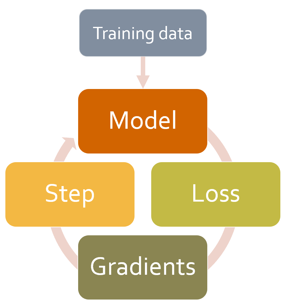
The usual way for deep learning practitioners to customize the training loop is to make a copy of an existing training loop, and then insert the code necessary for their particular changes into it. This is how nearly all code that you find online will look. But it has some very serious problems.
It's not very likely that some particular tweaked training loop is going to meet your particular needs. There are hundreds of changes that can be made to a training loop, which means there are billions and billions of possible permutations. You can't just copy one tweak from a training loop here, another from a training loop there, and expect them all to work together. Each will be based on different assumptions about the environment that it's working in, use different naming conventions, and expect the data to be in different formats.
We need a way to allow users to insert their own code at any part of the training loop, but in a consistent and well-defined way. Computer scientists have already come up with an elegant solution: the callback. A callback is a piece of code that you write, and inject into another piece of code at some predefined point. In fact, callbacks have been used with deep learning training loops for years. The problem is that in previous libraries it was only possible to inject code in a small subset of places where this may have been required, and, more importantly, callbacks were not able to do all the things they needed to do.
In order to be just as flexible as manually copying and pasting a training loop and directly inserting code into it, a callback must be able to read every possible piece of information available in the training loop, modify all of it as needed, and fully control when a batch, epoch, or even the whole training loop should be terminated. fastai is the first library to provide all of this functionality. It modifies the training loop so it looks like <<cb_loop>>.
深度学习从业者定制训练循环的通常方法是复制一个现有的训练循环,然后在其中插入他们特定变化所需的代码。这就是你在网上找到的几乎所有代码的样子。但是它有一些非常严重的问题。
某个经过调整的训练循环不太可能满足你的特殊需要。一个训练循环可以有数百种变化,这意味着有数十亿种可能的排列组合。你不能只是从这里的训练环路复制一个调整,从那里的训练环路复制另一个调整,并期望它们都能一起工作。每一个都会基于对它所处环境的不同假设,使用不同的命名规则,并期望数据采用不同的格式。
我们需要一种方法,允许用户在训练循环的任何部分插入他们自己的代码,但要以一致的、定义明确的方式。计算机科学家已经想出了一个优雅的解决方案:回调。回调是你写的一段代码,并在某个预定义的点注入另一段代码。事实上,回调已经在深度学习训练循环中使用了多年。问题是,在以前的库中,只能在一小部分可能需要的地方注入代码,而且更重要的是,回调不能做所有需要做的事情。
为了像手动复制和粘贴训练循环并直接插入代码一样灵活,回调必须能够读取训练循环中的每一个可能的信息,根据需要修改所有的信息,并完全控制一个批次、历时甚至整个训练循环应该何时终止。它修改了训练循环,使其看起来像<<cb_loop>>。
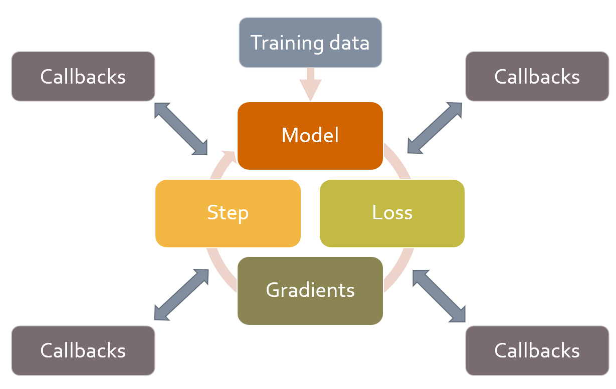
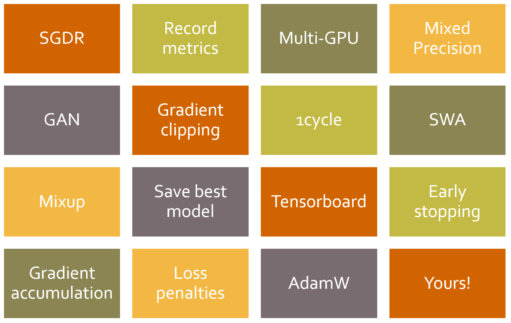
The real effectiveness of this approach has been borne out over the last couple of years—it has turned out that, by using the fastai callback system, we were able to implement every single new paper we tried and fulfilled every user request for modifying the training loop. The training loop itself has not required modifications. <<some_cbs>> shows just a few of the callbacks that have been added.
这种方法的真正有效性在过去几年中得到了证实--事实证明,通过使用fastai回调系统,我们能够实现我们尝试的每一篇新论文,并满足用户对修改训练循环的要求。训练循环本身不需要修改。<<some_cbs>>显示的只是一些已经添加的回调。
The reason that this is important is because it means that whatever idea we have in our head, we can implement it. We need never dig into the source code of PyTorch or fastai and hack together some one-off system to try out our ideas. And when we do implement our own callbacks to develop our own ideas, we know that they will work together with all of the other functionality provided by fastai–so we will get progress bars, mixed-precision training, hyperparameter annealing, and so forth.
Another advantage is that it makes it easy to gradually remove or add functionality and perform ablation studies. You just need to adjust the list of callbacks you pass along to your fit function.
这一点很重要,因为它意味着无论我们脑子里有什么想法,我们都可以实现它。我们不需要挖掘PyTorch或fastai的源代码,也不需要把一些一次性的系统砍掉来尝试我们的想法。当我们实现自己的回调来开发自己的想法时,我们知道它们将与fastai提供的所有其他功能一起工作,因此我们将得到进度条、混合精度训练、超参数退火等。
另一个优点是,它使逐步删除或增加功能和进行消融研究变得容易。你只需要调整你传递给你的拟合函数的回调列表。
As an example, here is the fastai source code that is run for each batch of the training loop:
try:
    self._split(b);                                  self('before_batch')
    self.pred = self.model(*self.xb);                self('after_pred')
    self.loss = self.loss_func(self.pred, *self.yb); self('after_loss')
    if not self.training: return
    self.loss.backward();                            self('after_backward')
    self.opt.step();                                 self('after_step')
    self.opt.zero_grad()
except CancelBatchException:                         self('after_cancel_batch')
finally:                                             self('after_batch')
The calls of the form self('...') are where the callbacks are called. As you see, this happens after every step. The callback will receive the entire state of training, and can also modify it. For instance, the input data and target labels are in self.xb and self.yb, respectively; a callback can modify these to alter the data the training loop sees. It can also modify self.loss, or even the gradients.
Let's see how this works in practice by writing a callback.
作为一个例子,这里是为训练循环的每个批次运行的fastai源代码:
try:
    self._split(b);                                  self('before_batch')
    self.pred = self.model(*self.xb);                self('after_pred')
    self.loss = self.loss_func(self.pred, *self.yb); self('after_loss')
    if not self.training: return
    self.loss.backward();                            self('after_backward')
    self.opt.step();                                 self('after_step')
    self.opt.zero_grad()
except CancelBatchException:                         self('after_cancel_batch')
finally: self('after_batch')self('...')形式的调用是回调被调用的地方。正如你所看到的,这发生在每个步骤之后。回调将接收整个训练的状态,也可以修改它。例如,输入数据和目标标签分别在self.xb和self.yb中;回调可以修改这些数据以改变训练循环看到的数据。它还可以修改self.loss,甚至是梯度。
让我们通过写一个回调来看看这在实践中是如何工作的。
Creating a Callback
创建一个回调
When you want to write your own callback, the full list of available events is:
before_fit:: called before doing anything; ideal for initial setup.before_epoch:: called at the beginning of each epoch; useful for any behavior you need to reset at each epoch.before_train:: called at the beginning of the training part of an epoch.before_batch:: called at the beginning of each batch, just after drawing said batch. It can be used to do any setup necessary for the batch (like hyperparameter scheduling) or to change the input/target before it goes into the model (for instance, apply Mixup).after_pred:: called after computing the output of the model on the batch. It can be used to change that output before it's fed to the loss function.after_loss:: called after the loss has been computed, but before the backward pass. It can be used to add penalty to the loss (AR or TAR in RNN training, for instance).after_backward:: called after the backward pass, but before the update of the parameters. It can be used to make changes to the gradients before said update (via gradient clipping, for instance).after_step:: called after the step and before the gradients are zeroed.after_batch:: called at the end of a batch, to perform any required cleanup before the next one.after_train:: called at the end of the training phase of an epoch.before_validate:: called at the beginning of the validation phase of an epoch; useful for any setup needed specifically for validation.after_validate:: called at the end of the validation part of an epoch.after_epoch:: called at the end of an epoch, for any cleanup before the next one.after_fit:: called at the end of training, for final cleanup.
The elements of this list are available as attributes of the special variable event, so you can just type event. and hit Tab in your notebook to see a list of all the options.
当你想写你自己的回调时,可用事件的完整列表是。
before_fit:: 在做任何事情之前被调用;非常适合初始设置。before_epoch:: 在每个周期的开始被调用;对任何需要在每个周期重置的行为都很有用。before_train::在一个历时的训练部分开始时调用。before_batch:: 在每个批次开始时调用,就在绘制该批次之后。它可以用来为批处理做任何必要的设置(如超参数调度),或者在进入模型之前改变输入/目标(例如,应用Mixup)。after_pred:: 在计算模型的输出后调用。它可以用来改变输出,然后再送入损失函数。after_loss::在计算完损失后,但在后向传递前调用。它可以用来给损失增加惩罚(例如,RNN训练中的AR或TAR)。after_backward::在后向传递之后,但在更新参数之前调用。它可以用来在更新前对梯度进行修改(例如通过梯度剪切)。after_step::在步骤之后,梯度归零之前调用。after_batch:在一个批次结束时调用,在下一个批次之前执行任何需要的清理工作。after_train:在一个epoch的训练阶段结束时调用。before_validate: 在一个历时的验证阶段开始时调用;对验证所需的任何设置很有用。after_validate: 在一个历时的验证部分结束时调用。after_epoch:在一个周期结束时调用,用于下一个周期前的任何清理工作。after_fit: 在训练结束时调用,用于最后的清理。
这个列表中的元素可以作为特殊变量event的属性,所以你可以在笔记本上输入event.,然后点击Tab,就可以看到所有选项的列表。
Let's take a look at an example. Do you recall how in <<chapter_nlp_dive>> we needed to ensure that our special reset method was called at the start of training and validation for each epoch? We used the ModelResetter callback provided by fastai to do this for us. But how does it work? Here's the full source code for that class:
让我们来看看一个例子。你还记得在<<chapter_nlp_dive>>中,我们需要确保我们的特殊reset方法在每个历时的训练和验证开始时被调用?我们使用了fastai提供的ModelResetter回调来做这件事。但它是如何工作的呢?下面是该类的完整源代码:
class ModelResetter(Callback):
    def before_train(self):    self.model.reset()
    def before_validate(self): self.model.reset()
Yes, that's actually it! It just does what we said in the preceding paragraph: after completing training or validation for an epoch, call a method named reset.
Callbacks are often "short and sweet" like this one. In fact, let's look at one more. Here's the fastai source for the callback that adds RNN regularization (AR and TAR):
是的,实际上就是这样! 它只是做了我们在前一段中所说的:在完成训练或验证一个epoch后,调用一个名为reset的方法。
回调通常像这个一样 "短小精悍"。事实上,让我们再看看一个。下面是增加RNN正则化(AR和TAR)的回调的fastai源。
class RNNRegularizer(Callback):
    def __init__(self, alpha=0., beta=0.): self.alpha,self.beta = alpha,beta

    def after_pred(self):
        self.raw_out,self.out = self.pred[1],self.pred[2]
        self.learn.pred = self.pred[0]

    def after_loss(self):
        if not self.training: return
        if self.alpha != 0.:
            self.learn.loss += self.alpha * self.out[-1].float().pow(2).mean()
        if self.beta != 0.:
            h = self.raw_out[-1]
            if len(h)>1:
                self.learn.loss += self.beta * (h[:,1:] - h[:,:-1]
                                               ).float().pow(2).mean()
note: Code It Yourself: Go back and reread "Activation Regularization and Temporal Activation Regularization" in <<chapter_nlp_dive>> then take another look at the code here. Make sure you understand what it's doing, and why.
注意:自己编写代码:回去重读<<chapter_nlp_dive>>中的 "激活正则化和时间激活正则化",然后再看一下这里的代码。确保你理解它在做什么,以及为什么。
In both of these examples, notice how we can access attributes of the training loop by directly checking self.model or self.pred. That's because a Callback will always try to get an attribute it doesn't have inside the Learner associated with it. These are shortcuts for self.learn.model or self.learn.pred. Note that they work for reading attributes, but not for writing them, which is why when RNNRegularizer changes the loss or the predictions you see self.learn.loss = or self.learn.pred = .
在这两个例子中,注意到我们如何通过直接检查self.model或self.pred来访问训练循环的属性。这是因为Callback总是试图获取它在与之相关的Learner中没有的属性。这些是self.learn.model或self.learn.pred的快捷方式。注意,它们对读取属性有效,但对写入属性无效,这就是为什么当RNNRegularizer改变损失或预测时,你会看到self.learn.loss = 或self.learn.pred = 。
When writing a callback, the following attributes of Learner are available:
model:: The model used for training/validation.data:: The underlyingDataLoaders.loss_func:: The loss function used.opt:: The optimizer used to update the model parameters.opt_func:: The function used to create the optimizer.cbs:: The list containing all theCallbacks.dl:: The currentDataLoaderused for iteration.x/xb:: The last input drawn fromself.dl(potentially modified by callbacks).xbis always a tuple (potentially with one element) andxis detuplified. You can only assign toxb.y/yb:: The last target drawn fromself.dl(potentially modified by callbacks).ybis always a tuple (potentially with one element) andyis detuplified. You can only assign toyb.pred:: The last predictions fromself.model(potentially modified by callbacks).loss:: The last computed loss (potentially modified by callbacks).n_epoch:: The number of epochs in this training.n_iter:: The number of iterations in the currentself.dl.epoch:: The current epoch index (from 0 ton_epoch-1).iter:: The current iteration index inself.dl(from 0 ton_iter-1).
The following attributes are added by TrainEvalCallback and should be available unless you went out of your way to remove that callback:
train_iter:: The number of training iterations done since the beginning of this trainingpct_train:: The percentage of training iterations completed (from 0. to 1.)training:: A flag to indicate whether or not we're in training mode
The following attribute is added by Recorder and should be available unless you went out of your way to remove that callback:
smooth_loss:: An exponentially averaged version of the training loss
当编写回调时,`学习者'的以下属性是可用的。
model:: 用于训练/验证的模型。data:: 底层的`DataLoaders'.loss_func:: 使用的损失函数。opt:: 用来更新模型参数的优化器。opt_func:: 用于创建优化器的函数。cbs:: 包含所有 "回调 "的列表。dl:: 当前用于迭代的`DataLoader'。x/xb:: 最后一次从self.dl提取的输入(可能被回调修改)。xb总是一个元组(可能有一个元素),x被分解。你只能对xb进行赋值。y/yb:: 从self.dl中抽取的最后一个目标(可能被回调修改)。yb总是一个元组(可能有一个元素),y被解构。你只能对yb进行赋值。pred:: 来自self.model的最后预测(可能被回调修改)。loss:: 最后一次计算的损失(可能被回调修改)。n_epoch:: 本次训练的历时数。n_iter:: 当前`self.dl'中的迭代次数。epoch:: 当前 epoch 索引(从 0 到n_epoch-1)。iter:: 当前self.dl中的迭代索引(从0到n_iter-1)。
以下属性是由TrainEvalCallback添加的,除非你不顾一切地删除该回调,否则应该是可用的。
train_iter:: 自本次训练开始以来所做的训练迭代的数量。pct_train:: 训练迭代完成的百分比(从0.到1.)。- 训练":: 一个标志,表示我们是否在训练模式中。
下面的属性是由Recorder添加的,应该是可用的,除非你不顾一切地删除那个回调。
smooth_loss:: 训练损失的指数平均化版本
Callbacks can also interrupt any part of the training loop by using a system of exceptions.
回调也可以通过使用一个异常系统来中断训练循环的任何部分。
Callback Ordering and Exceptions
回调排序和异常情况
Sometimes, callbacks need to be able to tell fastai to skip over a batch, or an epoch, or stop training altogether. For instance, consider TerminateOnNaNCallback. This handy callback will automatically stop training any time the loss becomes infinite or NaN (not a number). Here's the fastai source for this callback:
有时,回调需要能够告诉fastai跳过一个批次,或一个世代,或完全停止训练。例如,考虑TerminateOnNaNCallback。这个方便的回调将在损失变得无限大或NaN(不是一个数字)时自动停止训练。下面是这个回调的fastai源:
class TerminateOnNaNCallback(Callback):
    run_before=Recorder
    def after_batch(self):
        if torch.isinf(self.loss) or torch.isnan(self.loss):
            raise CancelFitException
The line raise CancelFitException tells the training loop to interrupt training at this point. The training loop catches this exception and does not run any further training or validation. The callback control flow exceptions available are:
CancelBatchException:: Skip the rest of this batch and go toafter_batch.CancelTrainException:: Skip the rest of the training part of the epoch and go toafter_train.CancelValidException:: Skip the rest of the validation part of the epoch and go toafter_validate.CancelEpochException:: Skip the rest of this epoch and go toafter_epoch.CancelFitException:: Interrupt training and go toafter_fit.
这一行 raise CancelFitException告诉训练循环在这一点上中断训练。训练循环捕捉到这个异常,就不会再运行任何进一步的训练或验证。可用的回调控制流异常是。
CancelBatchException:: 跳过这个批次的其余部分,转到after_batch。CancelTrainException:: 跳过其余的训练部分,转到after_train。CancelValidException:: 跳过历时的验证部分,转到after_validate。CancelEpochException:: 跳过这个世代的其余部分,转到after_epoch。CancelFitException:: 中断训练并转到after_fit。
You can detect if one of those exceptions has occurred and add code that executes right after with the following events:
after_cancel_batch:: Reached immediately after aCancelBatchExceptionbefore proceeding toafter_batchafter_cancel_train:: Reached immediately after aCancelTrainExceptionbefore proceeding toafter_trainafter_cancel_valid:: Reached immediately after aCancelValidExceptionbefore proceeding toafter_validafter_cancel_epoch:: Reached immediately after aCancelEpochExceptionbefore proceeding toafter_epochafter_cancel_fit:: Reached immediately after aCancelFitExceptionbefore proceeding toafter_fit
你可以检测是否发生了这些异常,并通过以下事件添加紧接着执行的代码。
after_cancel_batch:: 在发生CancelBatchException后立即到达,然后进行after_batch。after_cancel_train:: 在发生CancelTrainException后立即到达,然后进入after_train。after_cancel_valid:: 在发生CancelValidException后立即到达,然后进入after_valid。After_cancel_epoch:: 在发生CancelEpochException后立即到达,然后进入after_epoch。after_cancel_fit:: 在发生CancelFitException后立即到达,然后进入after_fit。
Sometimes, callbacks need to be called in a particular order. For example, in the case of TerminateOnNaNCallback, it's important that Recorder runs its after_batch after this callback, to avoid registering an NaN loss. You can specify run_before (this callback must run before ...) or run_after (this callback must run after ...) in your callback to ensure the ordering that you need.
有时,回调需要以特定的顺序被调用。例如,在TerminateOnNaNCallback的情况下,重要的是Recorder在这个回调之后运行它的after_batch,以避免注册一个NaN损失。你可以在回调中指定run_before(这个回调必须在...之前运行)或run_after(这个回调必须在...之后运行),以确保你需要的排序。
Conclusion
结论
In this chapter we took a close look at the training loop, exploring different variants of SGD and why they can be more powerful. At the time of writing, developing new optimizers is a very active area of research, so by the time you read this chapter there may be an addendum on the book's website that presents new variants. Be sure to check out how our general optimizer framework can help you implement new optimizers very quickly.
We also examined the powerful callback system that allows you to customize every bit of the training loop by enabling you to inspect and modify any parameter you like between each step.
在这一章中,我们仔细研究了训练循环,探索了SGD的不同变体,以及为什么它们可以更强大。在写这篇文章的时候,开发新的优化器是一个非常活跃的研究领域,所以当你读到这一章的时候,本书的网站上可能已经有了介绍新变体的附录。一定要看看我们的通用优化器框架如何帮助你快速实现新的优化器。
我们还研究了强大的回调系统,它使你能够在每一步之间检查和修改任何你喜欢的参数,从而定制训练循环的每一点。
Questionnaire
- What is the equation for a step of SGD, in math or code (as you prefer)?
- What do we pass to
vision_learnerto use a non-default optimizer? - What are optimizer callbacks?
- What does
zero_graddo in an optimizer? - What does
stepdo in an optimizer? How is it implemented in the general optimizer? - Rewrite
sgd_cbto use the+=operator, instead ofadd_. - What is "momentum"? Write out the equation.
- What's a physical analogy for momentum? How does it apply in our model training settings?
- What does a bigger value for momentum do to the gradients?
- What are the default values of momentum for 1cycle training?
- What is RMSProp? Write out the equation.
- What do the squared values of the gradients indicate?
- How does Adam differ from momentum and RMSProp?
- Write out the equation for Adam.
- Calculate the values of
unbias_avgandw.avgfor a few batches of dummy values. - What's the impact of having a high
epsin Adam? - Read through the optimizer notebook in fastai's repo, and execute it.
- In what situations do dynamic learning rate methods like Adam change the behavior of weight decay?
- What are the four steps of a training loop?
- Why is using callbacks better than writing a new training loop for each tweak you want to add?
- What aspects of the design of fastai's callback system make it as flexible as copying and pasting bits of code?
- How can you get the list of events available to you when writing a callback?
- Write the
ModelResettercallback (without peeking). - How can you access the necessary attributes of the training loop inside a callback? When can you use or not use the shortcuts that go with them?
- How can a callback influence the control flow of the training loop?
- Write the
TerminateOnNaNcallback (without peeking, if possible). - How do you make sure your callback runs after or before another callback?
调查问卷
- 在数学或代码中,SGD的一个步骤的方程式是什么(如你喜欢)?
- 为了使用一个非默认的优化器,我们应该向
vision_learner传递什么? - 什么是优化器的回调?
zero_grad在优化器中做什么?step在优化器中起什么作用?它在一般的优化器中是如何实现的?- 重写
sgd_cb以使用+=运算符,而不是add_。 - 什么是 "动量"?写出方程。
- 动量的物理比喻是什么?它在我们的模型训练环境中是如何应用的?
- 更大的动量值对梯度有什么作用?
- 1周期训练中动量的默认值是什么?
- 什么是RMSProp?写出方程。
- 梯度的平方值表示什么?
- 亚当与动量和RMSProp有什么不同?
- 写出亚当的方程式。
- 计算几批假值的
unbias_avg和w.avg的值。 - 在Adam中拥有一个高的`eps'有什么影响?
- 阅读fastai repo中的优化器笔记本,并执行它。
- 在什么情况下,像Adam这样的动态学习率方法会改变权重衰减的行为?
- 训练循环的四个步骤是什么?
- 为什么使用回调比为每一个你想添加的调整写一个新的训练循环更好?
- fastai的回调系统设计的哪些方面使它像复制和粘贴代码一样灵活?
- 写回调时,如何获得可用的事件列表?
- 编写
ModelResetter回调(不偷看)。 - 你如何在回调里面访问训练循环的必要属性?什么时候可以使用或不使用与之配套的快捷方式?
- 回调如何影响训练循环的控制流?
- 编写 "TerminateOnNaN "回调(如果可能,不要偷看)。
- 如何确保你的回调在另一个回调之后或之前运行?
Further Research
进一步研究
- Look up the "Rectified Adam" paper, implement it using the general optimizer framework, and try it out. Search for other recent optimizers that work well in practice, and pick one to implement.
- Look at the mixed-precision callback with the documentation. Try to understand what each event and line of code does.
- Implement your own version of the learning rate finder from scratch. Compare it with fastai's version.
- Look at the source code of the callbacks that ship with fastai. See if you can find one that's similar to what you're looking to do, to get some inspiration.
- 查阅 "Rectified Adam "的论文,用一般的优化器框架来实现它,并进行尝试。搜索其他最近在实践中运行良好的优化器,并挑选一个来实现。
- 用文档看一下混合精度回调。试着理解每个事件和每行代码的作用。
- 从头开始实现你自己版本的学习率查找器。将其与fastai的版本进行比较。
- 看一下fastai附带的回调的源代码。看看你是否能找到一个与你想做的事情相似的,以获得一些灵感。
Foundations of Deep Learning: Wrap up
深度学习的基础:总结
Congratulations, you have made it to the end of the "foundations of deep learning" section of the book! You now understand how all of fastai's applications and most important architectures are built, and the recommended ways to train them—and you have all the information you need to build these from scratch. While you probably won't need to create your own training loop, or batchnorm layer, for instance, knowing what is going on behind the scenes is very helpful for debugging, profiling, and deploying your solutions.
Since you understand the foundations of fastai's applications now, be sure to spend some time digging through the source notebooks and running and experimenting with parts of them. This will give you a better idea of how everything in fastai is developed.
In the next section, we will be looking even further under the covers: we'll explore how the actual forward and backward passes of a neural network are done, and we will see what tools are at our disposal to get better performance. We will then continue with a project that brings together all the material in the book, which we will use to build a tool for interpreting convolutional neural networks. Last but not least, we'll finish by building fastai's Learner class from scratch.
恭喜你,你已经走到了本书 "深度学习的基础 "部分的末尾!你现在明白了fastai的所有应用和最重要的架构是如何建立的,以及推荐的训练方法。你现在明白了fastai的所有应用和最重要的架构是如何建立的,以及推荐的训练方法--你拥有从头开始建立这些架构所需的所有信息。虽然你可能不需要创建你自己的训练循环,或批处理层,例如,知道幕后发生了什么,对调试、分析和部署你的解决方案非常有帮助。
既然你现在了解了fastai的应用基础,那么一定要花一些时间来挖掘源码笔记本,并对其中的部分内容进行运行和实验。这将使你更好地了解fastai的一切是如何开发的。
在下一节中,我们将更深入地研究:我们将探索神经网络的实际前向和后向传递是如何完成的,我们将看到有哪些工具可以让我们获得更好的性能。然后,我们将继续进行一个项目,将书中的所有材料汇集在一起,我们将用它来建立一个解释卷积神经网络的工具。最后但同样重要的是,我们将通过从头开始构建fastai的Learner类来结束。