
Chapter 14
ResNets
#hide
! [ -e /content ] && pip install -Uqq fastbook
import fastbook
fastbook.setup_book()#hide
from fastbook import *ResNets
In this chapter, we will build on top of the CNNs introduced in the previous chapter and explain to you the ResNet (residual network) architecture. It was introduced in 2015 by Kaiming He et al. in the article "Deep Residual Learning for Image Recognition" and is by far the most used model architecture nowadays. More recent developments in image models almost always use the same trick of residual connections, and most of the time, they are just a tweak of the original ResNet.
We will first show you the basic ResNet as it was first designed, then explain to you what modern tweaks make it more performant. But first, we will need a problem a little bit more difficult than the MNIST dataset, since we are already close to 100% accuracy with a regular CNN on it.
在本章中,我们将在上一章介绍的CNN之上进行构建,并向您解释ResNet(残差网络)架构。它是由Kaiming He等人于2015年在"用于图像识别的深度残差学习"一文中提出的,是迄今为止使用最多的模型架构。图像模型的最新发展几乎总是使用相同的残差连接技巧,大多数时候,它们只是对原始ResNet的一个微调。
我们将首先向您展示最初设计的基本ResNet,然后向您解释哪些现代调整使其性能更好。但首先,我们将需要一个比MNIST数据集更难的问题,上面有一个常规的CNN。
Going Back to Imagenette
回到Imagenette
It's going to be tough to judge any improvements we make to our models when we are already at an accuracy that is as high as we saw on MNIST in the previous chapter, so we will tackle a tougher image classification problem by going back to Imagenette. We'll stick with small images to keep things reasonably fast.
Let's grab the data—we'll use the already-resized 160 px version to make things faster still, and will random crop to 128 px:
当我们已经达到上一章在MNIST上看到的精度时,很难判断我们对模型所做的任何改进,所以我们将通过回到Imagenette来解决一个更难的图像分类问题。我们将坚持使用小图像以保持相当快的速度。
让我们获取数据—-我们将使用已经调整大小的160像素版本来使速度更快,并将随机裁剪到128像素:
def get_data(url, presize, resize):
    path = untar_data(url)
    return DataBlock(
        blocks=(ImageBlock, CategoryBlock), get_items=get_image_files,
        splitter=GrandparentSplitter(valid_name='val'),
        get_y=parent_label, item_tfms=Resize(presize),
        batch_tfms=[*aug_transforms(min_scale=0.5, size=resize),
                    Normalize.from_stats(*imagenet_stats)],
).dataloaders(path, bs=128)dls = get_data(URLs.IMAGENETTE_160, 160, 128)dls.show_batch(max_n=4)Output
<Figure size 432x432 with 4 Axes>
[省略较大 image/png 输出]
When we looked at MNIST we were dealing with 28×28-pixel images. For Imagenette we are going to be training with 128×128-pixel images. Later, we would like to be able to use larger images as well—at least as big as 224×224 pixels, the ImageNet standard. Do you recall how we managed to get a single vector of activations for each image out of the MNIST convolutional neural network?
The approach we used was to ensure that there were enough stride-2 convolutions such that the final layer would have a grid size of 1. Then we just flattened out the unit axes that we ended up with, to get a vector for each image (so, a matrix of activations for a mini-batch). We could do the same thing for Imagenette, but that would cause two problems:
- We'd need lots of stride-2 layers to make our grid 1×1 at the end—perhaps more than we would otherwise choose.
- The model would not work on images of any size other than the size we originally trained on.
One approach to dealing with the first of these issues would be to flatten the final convolutional layer in a way that handles a grid size other than 1×1. That is, we could simply flatten a matrix into a vector as we have done before, by laying out each row after the previous row. In fact, this is the approach that convolutional neural networks up until 2013 nearly always took. The most famous example is the 2013 ImageNet winner VGG, still sometimes used today. But there was another problem with this architecture: not only did it not work with images other than those of the same size used in the training set, but it required a lot of memory, because flattening out the convolutional layer resulted in many activations being fed into the final layers. Therefore, the weight matrices of the final layers were enormous.
This problem was solved through the creation of fully convolutional networks. The trick in fully convolutional networks is to take the average of activations across a convolutional grid. In other words, we can simply use this function:
当我们查看MNIST时,我们处理的是28×28像素的图像。对于Imagenette,我们将使用128×128像素的图像进行训练。之后,我们还希望能够使用更大的图像——至少是ImageNet标准的224×224像素。你还记得我们是如何从MNIST卷积神经网络中为每张图像获得一个激活向量的吗?
我们使用的方法是确保有足够的stride-2卷积,以使最后一层的网格大小为1。然后我们将最终得到的单位轴展平,以获得每个图像的向量(因此,一个小批量的激活矩阵)。我们可以对Imagenette做同样的事情,但这会导致两个问题:
- 我们需要大量的stride-2层来使我们的网格最终达到1×1——也许比我们选择的要多。
- 该模型不适用于我们最初训练的尺寸以外的任何尺寸的图像。
处理第一个问题的一种方法是,以处理1×1以外的网格大小的方式展平最终的卷积层。也就是说,我们可以像以前一样简单地将矩阵展平为向量,方法是将每一行放在前一行之后。事实上,直到 2013 年,卷积神经网络几乎总是采用这种方法。最著名的例子是2013年的ImageNet获胜者VGG,至今仍有使用。但这种架构还有另一个问题:它不仅不能处理训练集中使用的相同大小的图像之外的图像,而且需要大量内存,因为展平卷积层会导致许多激活被输入到最后一层。因此,最后一层的权重矩阵是巨大的。
这个问题是通过创建全卷积网络解决的。全卷积网络的诀窍是在卷积网格上取激活的平均值。换句话说,我们可以简单地使用这个函数:
def avg_pool(x): return x.mean((2,3))As you see, it is taking the mean over the x- and y-axes. This function will always convert a grid of activations into a single activation per image. PyTorch provides a slightly more versatile module called nn.AdaptiveAvgPool2d, which averages a grid of activations into whatever sized destination you require (although we nearly always use a size of 1).
A fully convolutional network, therefore, has a number of convolutional layers, some of which will be stride 2, at the end of which is an adaptive average pooling layer, a flatten layer to remove the unit axes, and finally a linear layer. Here is our first fully convolutional network:
如您所见,它在x轴和y轴上取平均值。这个函数将始终将激活网格转换为每张图像的单个激活。PyTorch提供了一个更通用的模块nn.AdaptiveAvgPool2d,它将激活网格平均到您需要的任何大小的目标(尽管我们几乎总是使用大小为1)。
因此,一个全卷积网络有许多卷积层,其中一些步幅为 2 ,最后是一个自适应平均池化层,一个用于去除单位轴的扁平层,最后是一个线性层。这是我们的第一个全卷积的网络:
def block(ni, nf): return ConvLayer(ni, nf, stride=2)
def get_model():
    return nn.Sequential(
        block(3, 16),
        block(16, 32),
        block(32, 64),
        block(64, 128),
        block(128, 256),
        nn.AdaptiveAvgPool2d(1),
        Flatten(),
        nn.Linear(256, dls.c))
We're going to be replacing the implementation of block in the network with other variants in a moment, which is why we're not calling it conv any more. We're also saving some time by taking advantage of fastai's ConvLayer, which that already provides the functionality of conv from the last chapter (plus a lot more!).
我们将在一会儿用其他变体替换网络中block的实现,这就是为什么我们不再称它为conv的原因。我们还通过利用fastai的ConvLayer来节省一些时间,它已经提供了上一章中conv功能(还有更多!)
stop: Consider this question: would this approach makes sense for an optical character recognition (OCR) problem such as MNIST? The vast majority of practitioners tackling OCR and similar problems tend to use fully convolutional networks, because that's what nearly everybody learns nowadays. But it really doesn't make any sense! You can't decide, for instance, whether a number is a 3 or an 8 by slicing it into small pieces, jumbling them up, and deciding whether on average each piece looks like a 3 or an 8. But that's what adaptive average pooling effectively does! Fully convolutional networks are only really a good choice for objects that don't have a single correct orientation or size (e.g., like most natural photos).
停止:考虑这个问题:这种方法对光学字符识别(OCR)问题(如MNIST)是否有意义?绝大多数处理OCR和类似问题的从业者倾向于使用全卷积网络,因为这是现在几乎每个人都在学习的东西。但这真的没有任何意义!例如,你不能通过将一个数字切成小块,把它们混在一起,并决定平均每个块看起来是3还是8来决定它是3还是8。但这就是自适应平均池有效做到的!对于没有单一正确方向或大小的对象(例如,像大多数自然照片一样),全卷积网络才是真正的好选择。
Once we are done with our convolutional layers, we will get activations of size bs x ch x h x w (batch size, a certain number of channels, height, and width). We want to convert this to a tensor of size bs x ch, so we take the average over the last two dimensions and flatten the trailing 1×1 dimension like we did in our previous model.
This is different from regular pooling in the sense that those layers will generally take the average (for average pooling) or the maximum (for max pooling) of a window of a given size. For instance, max pooling layers of size 2, which were very popular in older CNNs, reduce the size of our image by half on each dimension by taking the maximum of each 2×2 window (with a stride of 2).
As before, we can define a Learner with our custom model and then train it on the data we grabbed earlier:
一旦我们完成了卷积层,我们将获得大小为bs x ch x h x w(批大小,一定数量的通道,高度和宽度)的激活。我们想将其转换为大小为bs x ch的张量,因此我们取最后两个维度的平均值,并像在之前的模型中所做的那样将尾随的 1×1 维度展平。
这与常规池化不同,因为这些层通常会取给定大小的窗口的平均值(对于平均池化)或最大值(对于最大池化)。例如,大小为2的最大池化层,在旧CNN中非常流行,通过取每个2×2窗口的最大值(步幅为2),在每个维度上将我们的图像大小减少一半。
和之前一样,我们可以使用我们的自定义模型定义一个Learner,然后根据我们之前获取的数据对其进行训练:
def get_learner(m):
    return Learner(dls, m, loss_func=nn.CrossEntropyLoss(), metrics=accuracy
                  ).to_fp16()

learn = get_learner(get_model())learn.lr_find()Output
<IPython.core.display.HTML object>
(0.47863011360168456, 3.981071710586548)
<Figure size 432x288 with 1 Axes>

3e-3 is often a good learning rate for CNNs, and that appears to be the case here too, so let's try that:
3e-3对于CNN来说通常是一个很好的学习率,这里似乎也是如此,所以让我们尝试一下:
learn.fit_one_cycle(5, 3e-3)Output
<IPython.core.display.HTML object>
| epoch | train_loss | valid_loss | accuracy | time |
|---|---|---|---|---|
| 0 | 1.901582 | 2.155090 | 0.325350 | 00:07 |
| 1 | 1.559855 | 1.586795 | 0.507771 | 00:07 |
| 2 | 1.296350 | 1.295499 | 0.571720 | 00:07 |
| 3 | 1.144139 | 1.139257 | 0.639236 | 00:07 |
| 4 | 1.049770 | 1.092619 | 0.659108 | 00:07 |
That's a pretty good start, considering we have to pick the correct one of 10 categories, and we're training from scratch for just 5 epochs! We can do way better than this using a deeper mode, but just stacking new layers won't really improve our results (you can try and see for yourself!). To work around this problem, ResNets introduce the idea of skip connections. We'll explore those and other aspects of ResNets in the next section.
这是一个很好的开始,考虑到我们必须从10个类别中选择正确的一个,而且我们从头开始训练了5个epoch!我们可以使用更深的模式做得更好,但仅仅堆叠新层并不能真正改善我们的结果(你可以自己试试看!)为了解决这个问题,ResNets引入了跳过连接的概念。我们将在下一节中探索ResNets的这些和其他方面。
Building a Modern CNN: ResNet
构建现代CNN: ResNet
We now have all the pieces we need to build the models we have been using in our computer vision tasks since the beginning of this book: ResNets. We'll introduce the main idea behind them and show how it improves accuracy on Imagenette compared to our previous model, before building a version with all the recent tweaks.
我们现在拥有构建自本书开始以来一直在计算机视觉任务中使用的模型所需的所有部分:ResNets。我们将介绍它们背后的主要思想,并展示与我们以前的模型相比,它如何提高 Imagenette 的准确性,然后再构建一个包含所有最近调整的版本。
Skip Connections
跳过连接
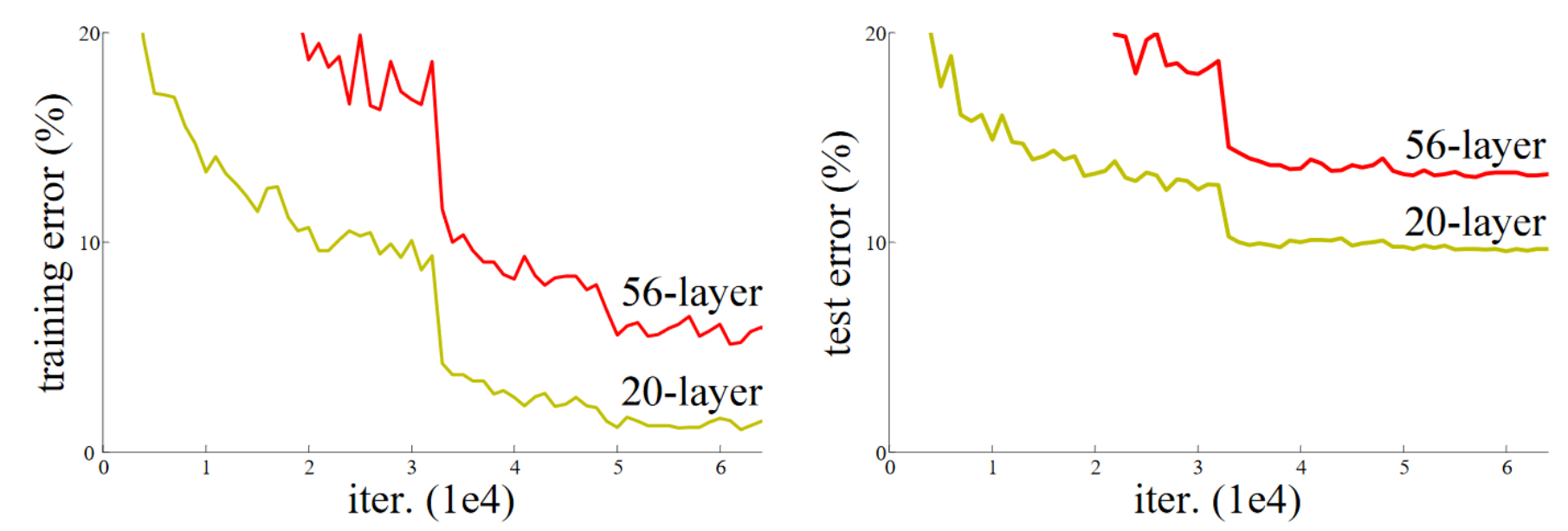
In 2015, the authors of the ResNet paper noticed something that they found curious. Even after using batchnorm, they saw that a network using more layers was doing less well than a network using fewer layers—and there were no other differences between the models. Most interestingly, the difference was observed not only in the validation set, but also in the training set; so, it wasn't just a generalization issue, but a training issue. As the paper explains:
: Unexpectedly, such degradation is not caused by overfitting, and adding more layers to a suitably deep model leads to higher training error, as [previously reported] and thoroughly verified by our experiments.
This phenomenon was illustrated by the graph in <<resnet_depth>>, with training error on the left and test error on the right.
2015年,ResNet论文的作者注意到一些他们感到好奇的事情。即使在使用batchnorm之后,他们也发现使用更多层的网络的表现不如使用更少层的网络——而且模型之间没有其他差异。最有趣的是,这种差异不仅在验证集中观察到,在训练集中也观察到;所以,这不仅仅是一个泛化问题,而是一个训练问题。正如论文所解释的:
:出乎意料的是,这种退化不是由过拟合引起的,并且向适当深度的模型添加更多层会导致更高的训练误差,正如[先前报道的]并由我们的实验彻底验证。
这种现象可以用<<resnet_depth>>中的图来说明,左边是训练误差,右边是测试误差。
As the authors mention here, they are not the first people to have noticed this curious fact. But they were the first to make a very important leap:
: Let us consider a shallower architecture and its deeper counterpart that adds more layers onto it. There exists a solution by construction to the deeper model: the added layers are identity mapping, and the other layers are copied from the learned shallower model.
As this is an academic paper this process is described in a rather inaccessible way, but the concept is actually very simple: start with a 20-layer neural network that is trained well, and add another 36 layers that do nothing at all (for instance, they could be linear layers with a single weight equal to 1, and bias equal to 0). The result will be a 56-layer network that does exactly the same thing as the 20-layer network, proving that there are always deep networks that should be at least as good as any shallow network. But for some reason, SGD does not seem able to find them.
jargon: Identity mapping: Returning the input without changing it at all. This process is performed by an identity function.
Actually, there is another way to create those extra 36 layers, which is much more interesting. What if we replaced every occurrence of conv(x) with x + conv(x), where conv is the function from the previous chapter that adds a second convolution, then a batchnorm layer, then a ReLU. Furthermore, recall that batchnorm does gamma*y + beta. What if we initialized gamma to zero for every one of those final batchnorm layers? Then our conv(x) for those extra 36 layers will always be equal to zero, which means x+conv(x) will always be equal to x.
What has that gained us? The key thing is that those 36 extra layers, as they stand, are an identity mapping, but they have parameters, which means they are trainable. So, we can start with our best 20-layer model, add these 36 extra layers which initially do nothing at all, and then fine-tune the whole 56-layer model. Those extra 36 layers can then learn the parameters that make them most useful.
The ResNet paper actually proposed a variant of this, which is to instead "skip over" every second convolution, so effectively we get x+conv2(conv1(x)). This is shown by the diagram in <<resnet_block>> (from the paper).
正如作者在这里提到的,他们不是第一个注意到这个奇怪事实的人。但他们是第一个做出非常重要的飞跃的人:
:让我们考虑一个较浅的架构及其在其上添加更多层的更深层次的对应物。通过构建更深层的模型存在一种解决方案:添加的层是恒等映射,其他层是从学习到的较浅模型中复制的。
由于这是一篇学术论文,这个过程以一种相当难以理解的方式描述,但概念实际上非常简单:从一个训练良好的20层神经网络开始,再添加另外36层什么都不做(例如,它们可能是线性层,单个权重等于1,偏差等于0)。结果将是一个56层网络,它做的事情与20层网络完全相同,证明总是有深度网络应该至少与任何浅网络一样好。但由于某种原因,SGD似乎无法找到它们。
术语:恒等映射:返回输入而不改变它。这个过程由一个恒等函数执行。
实际上,还有另一种方法来创建额外的36层,这更有趣。如果我们用x + conv(x)替换conv(x)的每一次出现,其中conv是上一章中添加第二个卷积的函数,然后是batchnorm层,然后是ReLU。此外,回想一下batchnorm计算的是gamma*y + beta。如果我们将最后一个batchnorm层的gamma初始化为0会怎样?那么我们对这些额外的36层的conv(x)将始终等于零,这意味着x+conv(x)将始终等于x。
这给我们带来了什么?关键是,这36个额外的层,就目前而言,是一个恒等映射,但它们有参数,这意味着它们是可训练的。所以,我们可以从我们最好的20层模型开始,添加这36个额外的层,这些层最初什么都不做,然后微调整个56层模型。这额外的36层可以学习使它们最有用的参数。
ResNet论文实际上提出了这种方法的一种变体,即每隔一个卷积“跳过”一次,因此我们有效地得到x+conv2(conv1(x))。这由<<resnet_block>>中的图表(来自论文)显示。
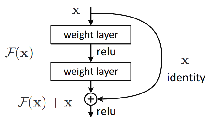
That arrow on the right is just the x part of x+conv2(conv1(x)), and is known as the identity branch or skip connection. The path on the left is the conv2(conv1(x)) part. You can think of the identity path as providing a direct route from the input to the output.
In a ResNet, we don't actually proceed by first training a smaller number of layers, and then adding new layers on the end and fine-tuning. Instead, we use ResNet blocks like the one in <<resnet_block>> throughout the CNN, initialized from scratch in the usual way, and trained with SGD in the usual way. We rely on the skip connections to make the network easier to train with SGD.
右边的箭头只是x+conv2(conv1(x))的x部分,被称为恒等分支或跳过连接。左边的路径是conv2(conv1(x))部分。您可以将恒等路径视为提供从输入到输出的直接路由。
在ResNet中,我们实际上并不是首先训练较少数量的层,然后在末尾添加新层并进行微调。相反,我们在整个 CNN 中使用像<<resnet_block>>中的 ResNet 块,以常规的方式从头开始初始化,并以常规的方式使用SGD进行训练。我们依靠跳过连接使SGD更容易训练网络。
There's another (largely equivalent) way to think of these ResNet blocks. This is how the paper describes it:
: Instead of hoping each few stacked layers directly fit a desired underlying mapping, we explicitly let these layers fit a residual mapping. Formally, denoting the desired underlying mapping as H(x), we let the stacked nonlinear layers fit another mapping of F(x) := H(x)−x. The original mapping is recast into F(x)+x. We hypothesize that it is easier to optimize the residual mapping than to optimize the original, unreferenced mapping. To the extreme, if an identity mapping were optimal, it would be easier to push the residual to zero than to fit an identity mapping by a stack of nonlinear layers.
Again, this is rather inaccessible prose—so let's try to restate it in plain English! If the outcome of a given layer is x, when using a ResNet block that returns y = x+block(x) we're not asking the block to predict y, we are asking it to predict the difference between y and x. So the job of those blocks isn't to predict certain features, but to minimize the error between x and the desired y. A ResNet is, therefore, good at learning about slight differences between doing nothing and passing though a block of two convolutional layers (with trainable weights). This is how these models got their name: they're predicting residuals (reminder: "residual" is prediction minus target).
One key concept that both of these two ways of thinking about ResNets share is the idea of ease of learning. This is an important theme. Recall the universal approximation theorem, which states that a sufficiently large network can learn anything. This is still true, but there turns out to be a very important difference between what a network can learn in principle, and what it is easy for it to learn with realistic data and training regimes. Many of the advances in neural networks over the last decade have been like the ResNet block: the result of realizing how to make something that was always possible actually feasible.
note: True Identity Path: The original paper didn't actually do the trick of using zero for the initial value of
gammain the last batchnorm layer of each block; that came a couple of years later. So, the original version of ResNet didn't quite begin training with a truly identity path through the ResNet blocks, but nonetheless having the ability to "navigate through" the skip connections did indeed make it train better. Adding the batchnormgammainit trick made the models train at even higher learning rates.
Here's the definition of a simple ResNet block (where norm_type=NormType.BatchZero causes fastai to init the gamma weights of the last batchnorm layer to zero):
还有另一种(基本上等价的)方式来思考这些ResNet块。这是论文对它的描述:
:我们不是希望每个堆叠的层都直接适合所需的底层映射,而是明确地让这些层适合残差映射。形式上,将所需的底层映射表示为H(x),我们让堆叠的非线性层适合F(x):=H(x)−x的另一个映射。原始映射被重铸为F(x)+x。我们假设优化残差映射比优化原始的、未引用的映射更容易。在极端情况下,如果一个恒等映射是最优的,那么将残差推到零要比用一堆非线性层来拟合恒等映射更容易。
同样,这是相当难以理解的散文——所以让我们试着用简单的英语重述它!如果给定层的结果是x,当使用返回y=x+block(x)的ResNet块时,我们不要求块预测y,而是要求它预测y和x之间的差异。所以这些块的工作不是预测某些特征,而是最小化x和所需y之间的误差。因此,ResNet 擅长学习什么都不做和通过一个由两个卷积层组成的块(具有可训练的权重)之间的细微差别。这就是这些模型的名字的由来:它们预测残差(提醒:残差是预测减去目标)。
这两种对ResNet的思考方式都有一个共同的关键概念,那就是易于学习的理念。这是一个重要的主题。回想一下通用近似定理,它指出一个足够大的网络可以学习任何东西。这仍然是正确的,但事实证明,一个网络在原则上可以学习的东西和它在通过现实数据和训练制度下容易学习的东西之间存在非常重要的区别。过去十年神经网络的许多进步就像ResNet块一样:实现如何使总是可能的事情变得实际可行的结果。
注意:True Identity Path:原始论文实际上并没有在每个块的最后一个batchnorm层中使用零作为
gamma的初始值;那是几年后的事情。因此,最初版本的ResNet并没有完全开始通过ResNet块的真正恒等路径进行训练,但尽管如此,具有“导航”跳过连接的能力确实使它训练得更好。加入batchnormgamma初始化技巧使模型以更高的学习率进行训练。
这是一个简单的ResNet块的定义(其中norm_type=NormType.BatchZero导致fastai将最后一个batchnorm层的gamma权重初始化为0):
class ResBlock(Module):
    def __init__(self, ni, nf):
        self.convs = nn.Sequential(
            ConvLayer(ni,nf),
            ConvLayer(nf,nf, norm_type=NormType.BatchZero))

    def forward(self, x): return x + self.convs(x)
There are two problems with this, however: it can't handle a stride other than 1, and it requires that ni==nf. Stop for a moment to think carefully about why this is.
The issue is that with a stride of, say, 2 on one of the convolutions, the grid size of the output activations will be half the size on each axis of the input. So then we can't add that back to x in forward because x and the output activations have different dimensions. The same basic issue occurs if ni!=nf: the shapes of the input and output connections won't allow us to add them together.
To fix this, we need a way to change the shape of x to match the result of self.convs. Halving the grid size can be done using an average pooling layer with a stride of 2: that is, a layer that takes 2×2 patches from the input and replaces them with their average.
Changing the number of channels can be done by using a convolution. We want this skip connection to be as close to an identity map as possible, however, which means making this convolution as simple as possible. The simplest possible convolution is one where the kernel size is 1. That means that the kernel is size ni*nf*1*1, so it's only doing a dot product over the channels of each input pixel—it's not combining across pixels at all. This kind of 1x1 convolution is very widely used in modern CNNs, so take a moment to think about how it works.
然而,这有两个问题:它不能处理1以外的步幅,并且需要ni==nf。停下来仔细想想为什么会这样。
问题是,在其中一个卷积上的步幅为2时,输出激活的网格大小将是输入每个轴上大小的一半。所以我们不能在forward中把它加回x,因为x和输出激活有不同的维度。同样的问题,如果ni!=nf:输入和输出连接的形状不允许我们将它们加在一起。
为了解决这个问题,我们需要一种方法来改变x的形状,以匹配self.convs的结果。可以使用步幅为 2 的平均池化层来将网格大小减半:也就是说,该层从输入中获取2×2个补丁,并用它们的平均值替换它们。
改变通道的数量可以通过使用卷积来完成。然而,我们希望这种跳过连接尽可能接近恒等映射,这意味着使这个卷积尽可能简单。最简单的卷积是核大小为1的卷积。这意味着内核的大小是ni*nf*1*1,所以它只对每个输入像素的通道做点积——它根本不跨像素组合。这种1x1卷积在现代CNN中应用非常广泛,所以花点时间思考一下它是如何工作的。
jargon: 1x1 convolution: A convolution with a kernel size of 1.
术语:1x1卷积:核大小为1的卷积。
Here's a ResBlock using these tricks to handle changing shape in the skip connection:
这是一个ResBlock使用这些技巧来处理跳过连接中的形状变化:
def _conv_block(ni,nf,stride):
    return nn.Sequential(
        ConvLayer(ni, nf, stride=stride),
ConvLayer(nf, nf, act_cls=None, norm_type=NormType.BatchZero))class ResBlock(Module):
def __init__(self, ni, nf, stride=1):
self.convs = _conv_block(ni,nf,stride)
self.idconv = noop if ni==nf else ConvLayer(ni, nf, 1, act_cls=None)
self.pool = noop if stride==1 else nn.AvgPool2d(2, ceil_mode=True)
def forward(self, x):
return F.relu(self.convs(x) + self.idconv(self.pool(x)))Note that we're using the noop function here, which simply returns its input unchanged (noop is a computer science term that stands for "no operation"). In this case, idconv does nothing at all if ni==nf, and pool does nothing if stride==1, which is what we wanted in our skip connection.
Also, you'll see that we've removed the ReLU (act_cls=None) from the final convolution in convs and from idconv, and moved it to after we add the skip connection. The thinking behind this is that the whole ResNet block is like a layer, and you want your activation to be after your layer.
Let's replace our block with ResBlock, and try it out:
请注意,我们这里使用的是noop函数,它只是返回其输入不变(noop是一个计算机科学术语,代表“无操作”)。在这种情况下,如果ni==nf,idconv什么也不做,如果stride==1, pool什么也不做,这是我们在跳过连接中想要的。
此外,您会看到我们已经从convs和idconv的最终卷积中删除了ReLU (act_cls=None),并将其移动到添加跳过连接后。这背后的想法是,整个ResNet块就像一个层,你希望你的激活在你的层之后。
让我们用ResBlock替换我们的block,并尝试一下:
def block(ni,nf): return ResBlock(ni, nf, stride=2)
learn = get_learner(get_model())learn.fit_one_cycle(5, 3e-3)Output
<IPython.core.display.HTML object>
| epoch | train_loss | valid_loss | accuracy | time |
|---|---|---|---|---|
| 0 | 1.973174 | 1.845491 | 0.373248 | 00:08 |
| 1 | 1.678627 | 1.778713 | 0.439236 | 00:08 |
| 2 | 1.386163 | 1.596503 | 0.507261 | 00:08 |
| 3 | 1.177839 | 1.102993 | 0.644841 | 00:09 |
| 4 | 1.052435 | 1.038013 | 0.667771 | 00:09 |
It's not much better. But the whole point of this was to allow us to train deeper models, and we're not really taking advantage of that yet. To create a model that's, say, twice as deep, all we need to do is replace our block with two ResBlocks in a row:
这也好不了多少。但这是为了让我们训练更深层次的模型,而我们还没有真正利用这一点。要创建一个深度两倍的模型,我们需要做的就是连续用两个ResBlock替换我们的block:
def block(ni, nf):
return nn.Sequential(ResBlock(ni, nf, stride=2), ResBlock(nf, nf))learn = get_learner(get_model())
learn.fit_one_cycle(5, 3e-3)Output
<IPython.core.display.HTML object>
| epoch | train_loss | valid_loss | accuracy | time |
|---|---|---|---|---|
| 0 | 1.964076 | 1.864578 | 0.355159 | 00:12 |
| 1 | 1.636880 | 1.596789 | 0.502675 | 00:12 |
| 2 | 1.335378 | 1.304472 | 0.588535 | 00:12 |
| 3 | 1.089160 | 1.065063 | 0.663185 | 00:12 |
| 4 | 0.942904 | 0.963589 | 0.692739 | 00:12 |
Now we're making good progress!
The authors of the ResNet paper went on to win the 2015 ImageNet challenge. At the time, this was by far the most important annual event in computer vision. We have already seen another ImageNet winner: the 2013 winners, Zeiler and Fergus. It is interesting to note that in both cases the starting points for the breakthroughs were experimental observations: observations about what layers actually learn, in the case of Zeiler and Fergus, and observations about which kinds of networks can be trained, in the case of the ResNet authors. This ability to design and analyze thoughtful experiments, or even just to see an unexpected result, say "Hmmm, that's interesting," and then, most importantly, set about figuring out what on earth is going on, with great tenacity, is at the heart of many scientific discoveries. Deep learning is not like pure mathematics. It is a heavily experimental field, so it's important to be a strong practitioner, not just a theoretician.
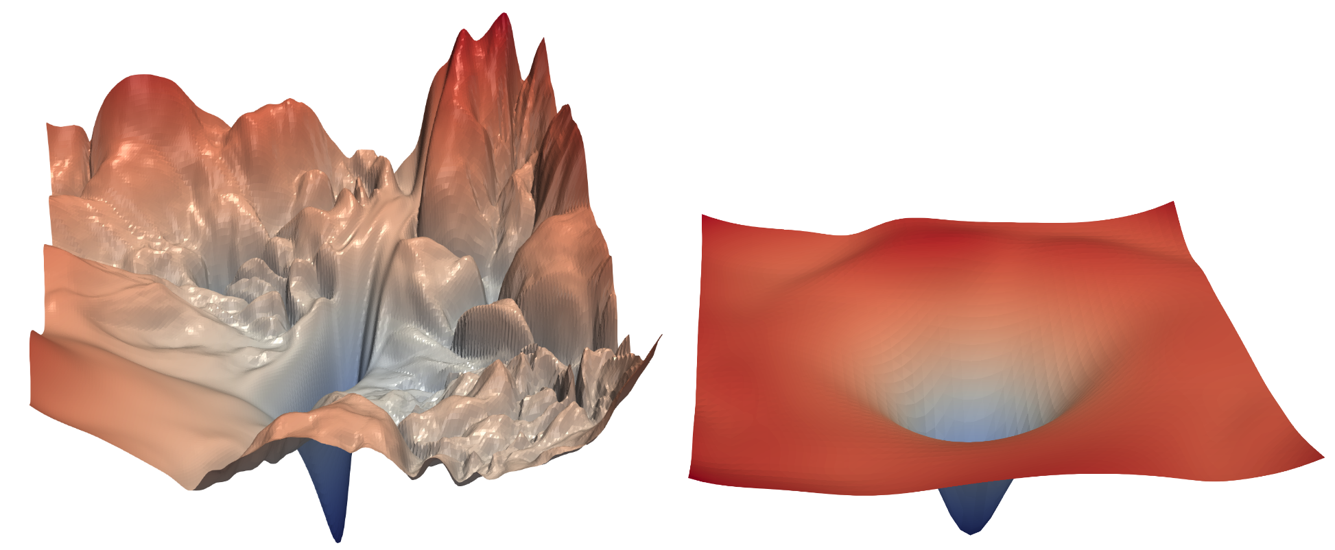
Since the ResNet was introduced, it's been widely studied and applied to many domains. One of the most interesting papers, published in 2018, is Hao Li et al.'s "Visualizing the Loss Landscape of Neural Nets". It shows that using skip connections helps smooth the loss function, which makes training easier as it avoids falling into a very sharp area. <<resnet_surface>> shows a stunning picture from the paper, illustrating the difference between the bumpy terrain that SGD has to navigate to optimize a regular CNN (left) versus the smooth surface of a ResNet (right).
现在我们正在取得良好的进展!
ResNet论文的作者后来赢得了2015年ImageNet挑战赛。当时,这是计算机视觉领域最重要的年度活动。我们已经看到了另一位ImageNet获奖者:2013年的获奖者,Zeiler和Fergus。有趣的是,在这两种情况下,取得突破的出发点都是实验观察:Zeiler和Fergus观察了哪些层实际上可以学习,ResNet的作者观察了哪些类型的网络可以训练。这种设计和分析深思熟虑的实验的能力,甚至只是为了看到一个意想不到的结果,说“嗯,这很有趣”,然后,最重要的是,以极大的毅力着手弄清楚到底发生了什么,这是许多科学发现的核心。深度学习不像纯数学。这是一个实验性很强的领域,所以做一个强大的实践者很重要,而不仅仅是一个理论家。
ResNet自问世以来,得到了广泛的研究和应用。2018 年发表的最有趣的论文之一是 Hao Li 等人的["可视化神经网络的损失景观"](https://arxiv.org/abs/1712.09913)。它表明,使用跳过连接有助于平滑损失函数,这使训练更容易,因为它避免落入一个非常尖锐的区域。<<resnet_surface>>展示了这篇论文中一张令人惊叹的图片,说明了SGD为优化常规CNN(左)而必须导航的颠簸地形与ResNet(右)的光滑表面之间的区别。
Our first model is already good, but further research has discovered more tricks we can apply to make it better. We'll look at those next.
我们的第一个模型已经很好了,但进一步的研究发现了更多我们可以应用的技巧来使它变得更好。我们接下来会看看这些。
A State-of-the-Art ResNet
最先进的ResNet
In "Bag of Tricks for Image Classification with Convolutional Neural Networks", Tong He et al. study different variations of the ResNet architecture that come at almost no additional cost in terms of number of parameters or computation. By using a tweaked ResNet-50 architecture and Mixup they achieved 94.6% top-5 accuracy on ImageNet, in comparison to 92.2% with a regular ResNet-50 without Mixup. This result is better than that achieved by regular ResNet models that are twice as deep (and twice as slow, and much more likely to overfit).
在["使用卷积神经网络进行图像分类的技巧包"](https://arxiv.org/abs/1812.01187)中,Tong He等人研究了ResNet架构的不同变体,这些变体在参数数量或计算方面几乎没有额外的成本。通过使用经过调整的ResNet-50架构和Mixup,他们在ImageNet上实现了94.6%的top-5准确度,相比之下,没有Mixup的常规ResNet-50的准确度为92.2%。这个结果比深度两倍的常规 ResNet 模型要好(慢两倍,而且更容易过拟合)。
jargon: top-5 accuracy: A metric testing how often the label we want is in the top 5 predictions of our model. It was used in the ImageNet competition because many of the images contained multiple objects, or contained objects that could be easily confused or may even have been mislabeled with a similar label. In these situations, looking at top-1 accuracy may be inappropriate. However, recently CNNs have been getting so good that top-5 accuracy is nearly 100%, so some researchers are using top-1 accuracy for ImageNet too now.
术语:top-5 accuracy:一个度量标准,测试我们想要的标签在我们模型的前 5 个预测中出现的频率。它在 ImageNet 比赛中被使用,因为许多图像包含多个对象,或者包含容易混淆的对象,甚至可能被错误地贴上了类似的标签。在这些情况下,只看top-1准确度可能是不合适的。然而,最近CNN变得如此之好,top-5 准确率接近 100%,所以一些研究人员现在也在ImageNet上使用top-1 准确率。
We'll use this tweaked version as we scale up to the full ResNet, because it's substantially better. It differs a little bit from our previous implementation, in that instead of just starting with ResNet blocks, it begins with a few convolutional layers followed by a max pooling layer. This is what the first layers, called the stem of the network, look like:
当我们扩展到完整的ResNet时,我们将使用这个调整后的版本,因为它要好得多。它与我们之前的实现有一点不同,它不是从ResNet块开始,而是从几个卷积层开始,然后是一个最大池化层。这是第一层,被称为网络的主干,是这样的:
def _resnet_stem(*sizes):
    return [
        ConvLayer(sizes[i], sizes[i+1], 3, stride = 2 if i==0 else 1)
            for i in range(len(sizes)-1)
] + [nn.MaxPool2d(kernel_size=3, stride=2, padding=1)]#hide_output
_resnet_stem(3,32,32,64)Output
[ConvLayer(
   (0): Conv2d(3, 32, kernel_size=(3, 3), stride=(2, 2), padding=(1, 1), bias=False)
   (1): BatchNorm2d(32, eps=1e-05, momentum=0.1, affine=True, track_running_stats=True)
   (2): ReLU()
 ), ConvLayer(
   (0): Conv2d(32, 32, kernel_size=(3, 3), stride=(1, 1), padding=(1, 1), bias=False)
   (1): BatchNorm2d(32, eps=1e-05, momentum=0.1, affine=True, track_running_stats=True)
   (2): ReLU()
 ), ConvLayer(
   (0): Conv2d(32, 64, kernel_size=(3, 3), stride=(1, 1), padding=(1, 1), bias=False)
   (1): BatchNorm2d(64, eps=1e-05, momentum=0.1, affine=True, track_running_stats=True)
   (2): ReLU()
 ), MaxPool2d(kernel_size=3, stride=2, padding=1, dilation=1, ceil_mode=False)]
[ConvLayer(
   (0): Conv2d(3, 32, kernel_size=(3, 3), stride=(2, 2), padding=(1, 1))
   (1): BatchNorm2d(32, eps=1e-05, momentum=0.1)
   (2): ReLU()
 ), ConvLayer(
   (0): Conv2d(32, 32, kernel_size=(3, 3), stride=(1, 1), padding=(1, 1))
   (1): BatchNorm2d(32, eps=1e-05, momentum=0.1)
   (2): ReLU()
 ), ConvLayer(
   (0): Conv2d(32, 64, kernel_size=(3, 3), stride=(1, 1), padding=(1, 1))
   (1): BatchNorm2d(64, eps=1e-05, momentum=0.1)
   (2): ReLU()
 ), MaxPool2d(kernel_size=3, stride=2, padding=1, ceil_mode=False)]
jargon: Stem: The first few layers of a CNN. Generally, the stem has a different structure than the main body of the CNN.
术语:Stem: CNN的前几层。通常,主干与CNN的主体有不同的结构。
The reason that we have a stem of plain convolutional layers, instead of ResNet blocks, is based on a very important insight about all deep convolutional neural networks: the vast majority of the computation occurs in the early layers. Therefore, we should keep the early layers as fast and simple as possible.
To see why so much computation occurs in the early layers, consider the very first convolution on a 128-pixel input image. If it is a stride-1 convolution, then it will apply the kernel to every one of the 128×128 pixels. That's a lot of work! In the later layers, however, the grid size could be as small as 4×4 or even 2×2, so there are far fewer kernel applications to do.
On the other hand, the first-layer convolution only has 3 input features and 32 output features. Since it is a 3×3 kernel, this is 3×32×3×3 = 864 parameters in the weights. But the last convolution will have 256 input features and 512 output features, resulting in 1,179,648 weights! So the first layers contain the vast majority of the computation, but the last layers contain the vast majority of the parameters.
A ResNet block takes more computation than a plain convolutional block, since (in the stride-2 case) a ResNet block has three convolutions and a pooling layer. That's why we want to have plain convolutions to start off our ResNet.
We're now ready to show the implementation of a modern ResNet, with the "bag of tricks." It uses four groups of ResNet blocks, with 64, 128, 256, then 512 filters. Each group starts with a stride-2 block, except for the first one, since it's just after a MaxPooling layer:
我们有一个纯卷积层而不是ResNet块的原因是基于对所有深度卷积神经网络的一个非常重要的见解:绝大多数计算发生在早期层。因此,我们应该尽可能保持早期层的快速和简单。
要了解为什么在早期层中会发生如此多的计算,请考虑128像素输入图像上的第一个卷积。如果它是步幅为1的卷积,那么它会将内核应用于 128×128 像素中的每一个像素。这是很多工作!然而,在后面的层中,网格的大小可能小到4×4甚至2×2,因此需要执行的内核应用程序要少得多。
另一方面,第一层卷积只有3个输入特征和32个输出特征。由于它是一个3×3的核,所以权重中有3×32×3×3 = 864个参数。但是最后一层卷积将有256个输入特征和512个输出特征,从而产生1,179,648个权重!所以第一层包含了绝大多数的计算,但最后一层包含了绝大多数的参数。
ResNet块比普通卷积块需要更多的计算,因为(在stride-2的情况下)ResNet块有三个卷积和一个池化层。这就是为什么我们希望使用简单的卷积来开始我们的 ResNet。
我们现在准备展示一个现代ResNet的实现,其中包含“技巧包”。它使用四组ResNet块,分别有64、128、256和512个过滤器。除了第一个,每组都以一个stride-2的块开始,因为它就在一个MaxPooling层之后:
class ResNet(nn.Sequential):
    def __init__(self, n_out, layers, expansion=1):
        stem = _resnet_stem(3,32,32,64)
        self.block_szs = [64, 64, 128, 256, 512]
        for i in range(1,5): self.block_szs[i] *= expansion
        blocks = [self._make_layer(*o) for o in enumerate(layers)]
        super().__init__(*stem, *blocks,
                         nn.AdaptiveAvgPool2d(1), Flatten(),
                         nn.Linear(self.block_szs[-1], n_out))

    def _make_layer(self, idx, n_layers):
        stride = 1 if idx==0 else 2
        ch_in,ch_out = self.block_szs[idx:idx+2]
        return nn.Sequential(*[
            ResBlock(ch_in if i==0 else ch_out, ch_out, stride if i==0 else 1)
            for i in range(n_layers)
        ])
The _make_layer function is just there to create a series of n_layers blocks. The first one is going from ch_in to ch_out with the indicated stride and all the others are blocks of stride 1 with ch_out to ch_out tensors. Once the blocks are defined, our model is purely sequential, which is why we define it as a subclass of nn.Sequential. (Ignore the expansion parameter for now; we'll discuss it in the next section. For now, it'll be 1, so it doesn't do anything.)
The various versions of the models (ResNet-18, -34, -50, etc.) just change the number of blocks in each of those groups. This is the definition of a ResNet-18:
_make_layer函数只是用来创建一系列n_layers块。第一个是从ch_in到ch_out的步幅,其他所有块都是步幅为1的块,有ch_out到ch_out张量。一旦块被定义,我们的模型就是纯顺序的,这就是为什么我们将其定义为nn.Sequential的子类。(暂不考虑expansion参数;我们将在下一节中讨论它。现在,它会是1,所以它什么都不做。)
模型的各种版本(ResNet-18、-34、-50等)只是更改每个组中的块数。这是ResNet-18的定义:
rn = ResNet(dls.c, [2,2,2,2])Let's train it for a little bit and see how it fares compared to the previous model:
让我们对其进行一些训练,看看它与之前的模型相比表现如何:
learn = get_learner(rn)
learn.fit_one_cycle(5, 3e-3)
Output
<IPython.core.display.HTML object>
| epoch | train_loss | valid_loss | accuracy | time |
|---|---|---|---|---|
| 0 | 1.673882 | 1.828394 | 0.413758 | 00:13 |
| 1 | 1.331675 | 1.572685 | 0.518217 | 00:13 |
| 2 | 1.087224 | 1.086102 | 0.650701 | 00:13 |
| 3 | 0.900428 | 0.968219 | 0.684331 | 00:12 |
| 4 | 0.760280 | 0.782558 | 0.757197 | 00:12 |
Even though we have more channels (and our model is therefore even more accurate), our training is just as fast as before, thanks to our optimized stem.
To make our model deeper without taking too much compute or memory, we can use another kind of layer introduced by the ResNet paper for ResNets with a depth of 50 or more: the bottleneck layer.
尽管我们有了更多的通道(因此我们的模型更加准确),但由于我们优化了主干,我们的训练仍和以前一样快。
为了在不占用太多计算或内存的情况下使我们的模型更深入,我们可以使用ResNet论文为深度为50或更多的ResNet引入的另一种层:瓶颈层。
Bottleneck Layers
瓶颈层
Instead of stacking two convolutions with a kernel size of 3, bottleneck layers use three different convolutions: two 1×1 (at the beginning and the end) and one 3×3, as shown on the right in <<resnet_compare>>.
瓶颈层不是堆叠内核大小为3的两个卷积,而是使用三个不同的卷积:两个1×1(在开头和结尾)和一个3×3,如<<resnet_compare>>中右侧所示。
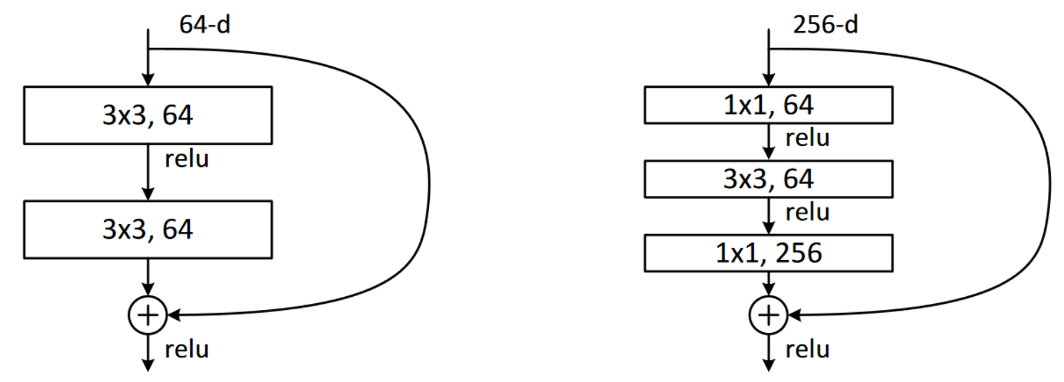
Why is that useful? 1×1 convolutions are much faster, so even if this seems to be a more complex design, this block executes faster than the first ResNet block we saw. This then lets us use more filters: as we see in the illustration, the number of filters in and out is 4 times higher (256 instead of 64) diminish then restore the number of channels (hence the name bottleneck). The overall impact is that we can use more filters in the same amount of time.
Let's try replacing our ResBlock with this bottleneck design:
为什么这很有用?1×1卷积要快得多,所以即使这看起来是一个更复杂的设计,这个块也比我们看到的第一个ResNet块执行得更快。这样我们就可以使用更多的过滤器:正如我们在插图中看到的,输入和输出的过滤器数量是原来的4倍(256而不是64),减少然后恢复通道数量(因此被称为瓶颈)。总体影响是我们可以在相同的时间内使用更多的过滤器。
让我们尝试用这个瓶颈设计替换我们的ResBlock:
def _conv_block(ni,nf,stride):
    return nn.Sequential(
        ConvLayer(ni, nf//4, 1),
        ConvLayer(nf//4, nf//4, stride=stride),
        ConvLayer(nf//4, nf, 1, act_cls=None, norm_type=NormType.BatchZero))
We'll use this to create a ResNet-50 with group sizes of (3,4,6,3). We now need to pass 4 in to the expansion parameter of ResNet, since we need to start with four times less channels and we'll end with four times more channels.
Deeper networks like this don't generally show improvements when training for only 5 epochs, so we'll bump it up to 20 epochs this time to make the most of our bigger model. And to really get great results, let's use bigger images too:
我们将使用它来创建一个组大小为(3,4,6,3)的ResNet-50。我们现在需要将4传递到ResNet的expansion参数,因为我们需要从少四倍的通道开始,然后以多四倍的通道结束。
像这样的更深的网络在只训练 5 个 epoch 时通常不会显示出改进,所以我们这次将把它增加到20个epoch,以充分利用我们更大的模型。为了真正获得更好的效果,让我们也使用更大的图像:
dls = get_data(URLs.IMAGENETTE_320, presize=320, resize=224)We don't have to do anything to account for the larger 224-pixel images; thanks to our fully convolutional network, it just works. This is also why we were able to do progressive resizing earlier in the book—the models we used were fully convolutional, so we were even able to fine-tune models trained with different sizes. We can now train our model and see the effects:
我们不需要做任何事情来解释224像素的大图像;多亏了我们的全卷积网络,它就可以工作了。这也是为什么我们能够在本书前面部分进行渐进式调整大小的原因——我们使用的模型是全卷积的,所以我们甚至能够微调用不同大小训练的模型。现在我们可以训练我们的模型并看到效果:
rn = ResNet(dls.c, [3,4,6,3], 4)learn = get_learner(rn)
learn.fit_one_cycle(20, 3e-3)Output
<IPython.core.display.HTML object>
| epoch | train_loss | valid_loss | accuracy | time |
|---|---|---|---|---|
| 0 | 1.613448 | 1.473355 | 0.514140 | 00:31 |
| 1 | 1.359604 | 2.050794 | 0.397452 | 00:31 |
| 2 | 1.253112 | 4.511735 | 0.387006 | 00:31 |
| 3 | 1.133450 | 2.575221 | 0.396178 | 00:31 |
| 4 | 1.054752 | 1.264525 | 0.613758 | 00:32 |
| 5 | 0.927930 | 2.670484 | 0.422675 | 00:32 |
| 6 | 0.838268 | 1.724588 | 0.528662 | 00:32 |
| 7 | 0.748289 | 1.180668 | 0.666497 | 00:31 |
| 8 | 0.688637 | 1.245039 | 0.650446 | 00:32 |
| 9 | 0.645530 | 1.053691 | 0.674904 | 00:31 |
| 10 | 0.593401 | 1.180786 | 0.676433 | 00:32 |
| 11 | 0.536634 | 0.879937 | 0.713885 | 00:32 |
| 12 | 0.479208 | 0.798356 | 0.741656 | 00:32 |
| 13 | 0.440071 | 0.600644 | 0.806879 | 00:32 |
| 14 | 0.402952 | 0.450296 | 0.858599 | 00:32 |
| 15 | 0.359117 | 0.486126 | 0.846369 | 00:32 |
| 16 | 0.313642 | 0.442215 | 0.861911 | 00:32 |
| 17 | 0.294050 | 0.485967 | 0.853503 | 00:32 |
| 18 | 0.270583 | 0.408566 | 0.875924 | 00:32 |
| 19 | 0.266003 | 0.411752 | 0.872611 | 00:33 |
We're getting a great result now! Try adding Mixup, and then training this for a hundred epochs while you go get lunch. You'll have yourself a very accurate image classifier, trained from scratch.
The bottleneck design we've shown here is typically only used in ResNet-50, -101, and -152 models. ResNet-18 and -34 models usually use the non-bottleneck design seen in the previous section. However, we've noticed that the bottleneck layer generally works better even for the shallower networks. This just goes to show that the little details in papers tend to stick around for years, even if they're actually not quite the best design! Questioning assumptions and "stuff everyone knows" is always a good idea, because this is still a new field, and there are lots of details that aren't always done well.
我们现在得到了一个很好的结果!试着添加Mixup,然后在你去吃午饭的时候训练它一百个 epoch。您将拥有一个非常准确的图像分类器,从头开始训练。
我们在这里展示的瓶颈设计通常只在ResNet-50、-101和-152模型中使用。ResNet-18和-34模型通常使用上一节中看到的非瓶颈设计。然而,我们注意到,即使对于较浅的网络,瓶颈层通常也能更好地工作。这只是表明,论文中的小细节往往会保留多年,即使它们实际上不是最好的设计!质疑假设和“每个人都知道的东西”总是一个好主意,因为这仍然是一个新的领域,而且有很多细节并不总是做得很好。
Conclusion
结论
You have now seen how the models we have been using for computer vision since the first chapter are built, using skip connections to allow deeper models to be trained. Even if there has been a lot of research into better architectures, they all use one version or another of this trick, to make a direct path from the input to the end of the network. When using transfer learning, the ResNet is the pretrained model. In the next chapter, we will look at the final details of how the models we actually used were built from it.
现在您已经看到了自第一章以来我们一直用于计算机视觉的模型是如何构建的,使用跳过连接来允许更深层次的模型被训练。即使已经有很多关于更好的架构的研究,它们都使用这种技巧的一个或另一个版本,来创建从输入到网络末端的直接路径。在使用迁移学习时,ResNet是预训练的模型。在下一章中,我们将会看到我们实际使用的模型是如何基于它构建的最终细节。
Questionnaire
问卷调查
- How did we get to a single vector of activations in the CNNs used for MNIST in previous chapters? Why isn't that suitable for Imagenette?
- What do we do for Imagenette instead?
- What is "adaptive pooling"?
- What is "average pooling"?
- Why do we need
Flattenafter an adaptive average pooling layer? - What is a "skip connection"?
- Why do skip connections allow us to train deeper models?
- What does <<resnet_depth>> show? How did that lead to the idea of skip connections?
- What is "identity mapping"?
- What is the basic equation for a ResNet block (ignoring batchnorm and ReLU layers)?
- What do ResNets have to do with residuals?
- How do we deal with the skip connection when there is a stride-2 convolution? How about when the number of filters changes?
- How can we express a 1×1 convolution in terms of a vector dot product?
- Create a
1x1 convolutionwithF.conv2dornn.Conv2dand apply it to an image. What happens to theshapeof the image? - What does the
noopfunction return? - Explain what is shown in <<resnet_surface>>.
- When is top-5 accuracy a better metric than top-1 accuracy?
- What is the "stem" of a CNN?
- Why do we use plain convolutions in the CNN stem, instead of ResNet blocks?
- How does a bottleneck block differ from a plain ResNet block?
- Why is a bottleneck block faster?
- How do fully convolutional nets (and nets with adaptive pooling in general) allow for progressive resizing?
- 在前面的章节中,我们是如何得到用于MNIST的CNN中的单个激活向量的?为什么这不适合Imagenette?
- 我们为Imagenette做什么?
- 什么是“自适应池化”?
- 什么是“平均池化”?
- 为什么在自适应平均池化层之后我们需要
Flatten? - 什么是“跳过连接”?
- 为什么跳过连接允许我们训练更深的模型?
- <<resnet_depth>>显示什么?这是如何导致跳过连接的想法的?
- 什么是“恒等映射”?
- ResNet块(忽略batchnorm和ReLU层)的基本方程是什么?
- ResNet与残差有什么关系?
- 当存在 stride-2 卷积时,我们如何处理跳过连接?当过滤器的数量发生变化时如何?
- 我们如何用向量点积表示1×1卷积?
- 用
F.conv2d或nn.Conv2d创建一个1x1 convolution并将其应用到图像上。图像的shape会发生什么变化? noop函数返回什么?- 解释<<resnet_surface>>中显示的内容。
- 什么时候前5名的准确度比前1名的准确度更好?
- CNN的“主干”是什么?
- 为什么我们在CNN主干中使用简单的卷积,而不是ResNet块?
- 瓶颈块与普通的ResNet块有何不同?
- 为什么瓶颈块更快?
- 全卷积网络(以及一般具有自适应池化的网络)如何允许渐进调整大小?
Further Research
进一步的研究
- Try creating a fully convolutional net with adaptive average pooling for MNIST (note that you'll need fewer stride-2 layers). How does it compare to a network without such a pooling layer?
- In <<chapter_foundations>> we introduce Einstein summation notation. Skip ahead to see how this works, and then write an implementation of the 1×1 convolution operation using
torch.einsum. Compare it to the same operation usingtorch.conv2d. - Write a "top-5 accuracy" function using plain PyTorch or plain Python.
- Train a model on Imagenette for more epochs, with and without label smoothing. Take a look at the Imagenette leaderboards and see how close you can get to the best results shown. Read the linked pages describing the leading approaches.
- 尝试为MNIST创建一个具有自适应平均池化的全卷积网络(注意,您将需要更少的stride-2层)。它与没有这种池化层的网络相比如何?
- 在<<chapter_foundations>>中,我们引入了爱因斯坦求和符号。跳过来看看它是如何工作的,然后使用
torch.einsum编写1×1卷积操作的实现。将其与使用torch.conv2d的相同操作进行比较。 - 使用纯PyTorch或纯Python编写“top-5 accuracy”函数。
- 在Imagenette上训练模型以适应更多的epoch,使用和不使用标签平滑。看看Imagenette排行榜,看看你有多接近最佳结果。阅读描述主要方法的链接页面。