
Chapter 13
Convolutional Neural Networks
#hide
! [ -e /content ] && pip install -Uqq fastbook
import fastbook
fastbook.setup_book()#hide
from fastai.vision.all import *
from fastbook import *
matplotlib.rc('image', cmap='Greys')Convolutional Neural Networks
卷积神经网络
In <<chapter_mnist_basics>> we learned how to create a neural network recognizing images. We were able to achieve a bit over 98% accuracy at distinguishing 3s from 7s—but we also saw that fastai's built-in classes were able to get close to 100%. Let's start trying to close the gap.
In this chapter, we will begin by digging into what convolutions are and building a CNN from scratch. We will then study a range of techniques to improve training stability and learn all the tweaks the library usually applies for us to get great results.
在<<chapter_mnist_basics>>中,我们学习了如何创建一个神经网络来识别图像。我们能够在从7中区分3上达到98%以上的准确率——但我们也看到fastai的内置类能够接近100%。让我们开始尝试缩小差距。
在本章中,我们将首先深入研究卷积是什么,并从头开始构建CNN。然后,我们将研究一系列技术来提高训练的稳定性,并学习库通常为我们应用的所有调整以获得良好的结果。
The Magic of Convolutions
卷积的魔力
One of the most powerful tools that machine learning practitioners have at their disposal is feature engineering. A feature is a transformation of the data which is designed to make it easier to model. For instance, the add_datepart function that we used for our tabular dataset preprocessing in <<chapter_tabular>> added date features to the Bulldozers dataset. What kinds of features might we be able to create from images?
机器学习实践者拥有的最强大的工具之一是特征工程。特征是数据的转换,旨在使其更容易建模。例如,我们在<<chapter_tabular>>中用于表格数据集预处理的add_datepart函数为tabular数据集添加了日期特征。我们可以从图像中创建什么类型的特征?
jargon: Feature engineering: Creating new transformations of the input data in order to make it easier to model.
术语:特征工程:创建输入数据的新转换,以便更容易建模。
In the context of an image, a feature is a visually distinctive attribute. For example, the number 7 is characterized by a horizontal edge near the top of the digit, and a top-right to bottom-left diagonal edge underneath that. On the other hand, the number 3 is characterized by a diagonal edge in one direction at the top left and bottom right of the digit, the opposite diagonal at the bottom left and top right, horizontal edges at the middle, top, and bottom, and so forth. So what if we could extract information about where the edges occur in each image, and then use that information as our features, instead of raw pixels?
It turns out that finding the edges in an image is a very common task in computer vision, and is surprisingly straightforward. To do it, we use something called a convolution. A convolution requires nothing more than multiplication, and addition—two operations that are responsible for the vast majority of work that we will see in every single deep learning model in this book!
A convolution applies a kernel across an image. A kernel is a little matrix, such as the 3×3 matrix in the top right of <<basic_conv>>.
在图像的上下文中,特征是视觉上独特的属性。例如,数字7的特征是在数字顶部附近有一条水平边缘,在其下方有一条右上角到左下角的对角边缘。另一方面,数字3的特征是在数字的左上角和右下角的一个方向上的对角线边缘,左下角和右上角的对角线,中间、顶部和底部的水平边缘,等等。那么,如果我们可以提取关于边缘在每个图像中出现的位置的信息,然后将这些信息作为我们的特征,而不是原始像素呢?
事实证明,在计算机视觉中,寻找图像中的边缘是一项非常常见的任务,而且非常简单。为了做到这一点,我们使用了一种叫做卷积的方法。卷积只需要乘法和加法——这两个运算是本书中每一个深度学习模型中最重要的部分!
卷积将核应用于图像。卷积核是一个小矩阵,例如<<basic_conv>>右上角的3×3矩阵。
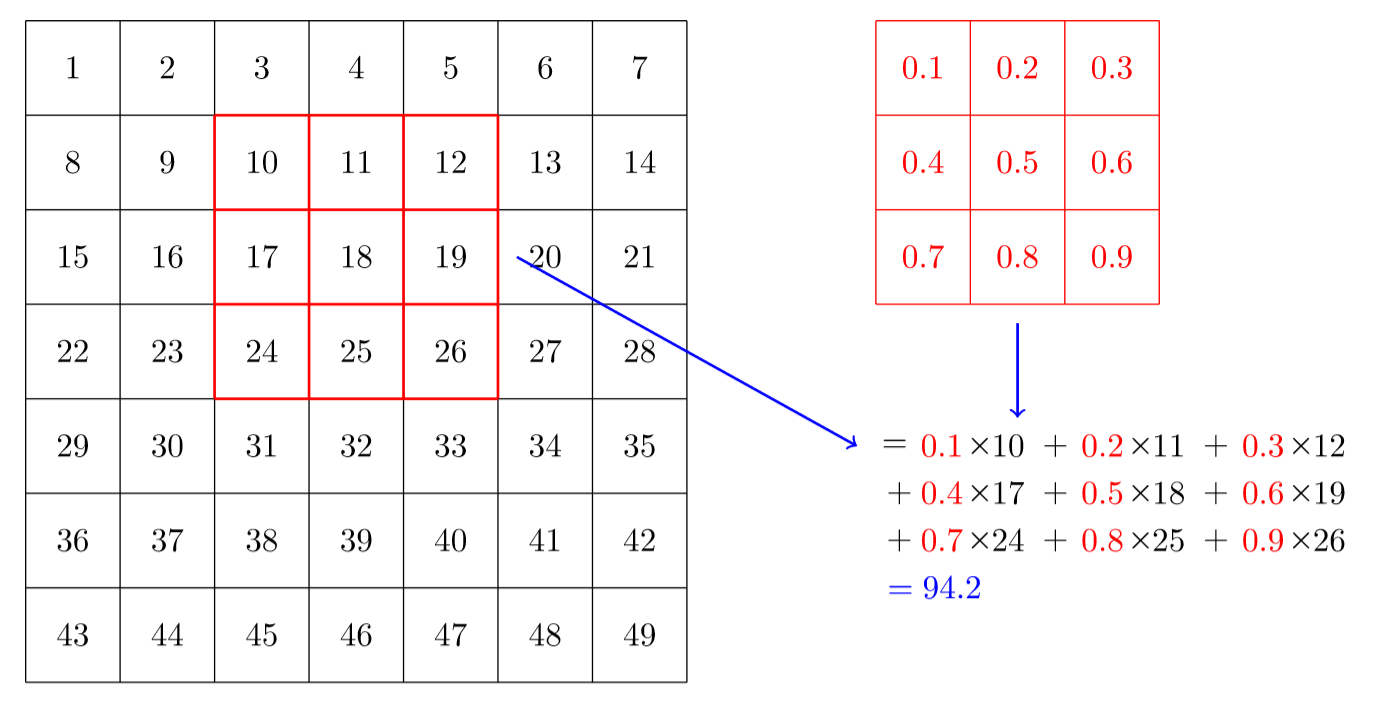
The 7×7 grid to the left is the image we're going to apply the kernel to. The convolution operation multiplies each element of the kernel by each element of a 3×3 block of the image. The results of these multiplications are then added together. The diagram in <<basic_conv>> shows an example of applying a kernel to a single location in the image, the 3×3 block around cell 18.
Let's do this with code. First, we create a little 3×3 matrix like so:
左边的7×7网格是我们将应用卷积核的图像。卷积运算将卷积核的每个元素乘以图像3×3块的每个元素。然后将这些乘法的结果相加。<<basic_conv>>中的图表显示了将卷积核应用于图像中单个位置(单元格18附近的3×3块)的示例。
让我们用代码来做到这一点。首先,我们创建一个3×3的小矩阵,如下所示:
top_edge = tensor([[-1,-1,-1],
                   [ 0, 0, 0],
                   [ 1, 1, 1]]).float()
We're going to call this our kernel (because that's what fancy computer vision researchers call these). And we'll need an image, of course:
我们将把它称为我们的卷积核(因为这是高级计算机视觉研究人员所称的)。当然,我们需要一张图像:
path = untar_data(URLs.MNIST_SAMPLE)#hide
Path.BASE_PATH = pathim3 = Image.open(path/'train'/'3'/'12.png')
show_image(im3);Output
<Figure size 72x72 with 1 Axes>

Now we're going to take the top 3×3-pixel square of our image, and multiply each of those values by each item in our kernel. Then we'll add them up, like so:
现在我们将取图像的顶部3×3像素正方形,并将这些值乘以卷积核中的每一项。然后我们将它们相加,如下所示:
im3_t = tensor(im3)
im3_t[0:3,0:3] * top_edge
Output
tensor([[-0., -0., -0.],
        [0., 0., 0.],
[0., 0., 0.]])(im3_t[0:3,0:3] * top_edge).sum()Output
tensor(0.)
Not very interesting so far—all the pixels in the top-left corner are white. But let's pick a couple of more interesting spots:
到目前为止还不是很有趣——左上角的所有像素都是白色的。但是让我们选择几个更有趣的地方:
#hide_output
df = pd.DataFrame(im3_t[:10,:20])
df.style.set_properties(**{'font-size':'6pt'}).background_gradient('Greys')
Output
<pandas.io.formats.style.Styler at 0x7fb709e80750>
| 0 | 1 | 2 | 3 | 4 | 5 | 6 | 7 | 8 | 9 | 10 | 11 | 12 | 13 | 14 | 15 | 16 | 17 | 18 | 19 | |
|---|---|---|---|---|---|---|---|---|---|---|---|---|---|---|---|---|---|---|---|---|
| 0 | 0 | 0 | 0 | 0 | 0 | 0 | 0 | 0 | 0 | 0 | 0 | 0 | 0 | 0 | 0 | 0 | 0 | 0 | 0 | 0 |
| 1 | 0 | 0 | 0 | 0 | 0 | 0 | 0 | 0 | 0 | 0 | 0 | 0 | 0 | 0 | 0 | 0 | 0 | 0 | 0 | 0 |
| 2 | 0 | 0 | 0 | 0 | 0 | 0 | 0 | 0 | 0 | 0 | 0 |
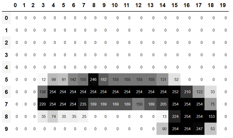
There's a top edge at cell 5,8. Let's repeat our calculation there:
在单元格5,8处有一条上边缘。让我们在那里重复我们的计算:
(im3_t[4:7,6:9] * top_edge).sum()Output
tensor(762.)
There's a right edge at cell 8,18. What does that give us?:
在单元格8,18处有一条右边缘。这给了我们什么?:
(im3_t[7:10,17:20] * top_edge).sum()Output
tensor(-29.)
As you can see, this little calculation is returning a high number where the 3×3-pixel square represents a top edge (i.e., where there are low values at the top of the square, and high values immediately underneath). That's because the -1 values in our kernel have little impact in that case, but the 1 values have a lot.
Let's look a tiny bit at the math. The filter will take any window of size 3×3 in our images, and if we name the pixel values like this:
it will return . If we are in a part of the image where , , and add up to the same as , , and , then the terms will cancel each other out and we will get 0. However, if is greater than , is greater than , and is greater than , we will get a bigger number as a result. So this filter detects horizontal edges—more precisely, edges where we go from bright parts of the image at the top to darker parts at the bottom.
Changing our filter to have the row of 1s at the top and the -1s at the bottom would detect horizontal edges that go from dark to light. Putting the 1s and -1s in columns versus rows would give us filters that detect vertical edges. Each set of weights will produce a different kind of outcome.
Let's create a function to do this for one location, and check it matches our result from before:
如您所见,这个小计算返回一个大数值,其中3×3像素的正方形代表上边缘(即,在正方形顶部有低值,紧接在其下方有高值)。这是因为在这种情况下,内核中的-1值影响很小,而1值影响很大。
让我们看一下数学。过滤器将在我们的图像中获取任何大小为3×3的窗口,如果我们将像素值命名为如下所示:
返回结果为。如果我们在图像的一部分,、和加起来与、和相同,那么这些项就会相互抵消,我们将得到0。但是,如果大于,大于,大于,我们将得到一个更大的数字。因此,该过滤器检测水平边缘——更准确地说,是从图像顶部明亮部分到底部较暗部分的边缘。
将过滤器更改为顶部的1s行和底部的-1s行,将检测从暗到亮的水平边缘。将1s和-1s放在列和行中将为我们提供检测垂直边缘的过滤器。每组权重都会产生不同类型的结果。
让我们创建一个函数来为一个位置执行此操作,并检查它是否与我们之前的结果匹配:
def apply_kernel(row, col, kernel):
return (im3_t[row-1:row+2,col-1:col+2] * kernel).sum()apply_kernel(5,7,top_edge)Output
tensor(762.)
But note that we can't apply it to the corner (e.g., location 0,0), since there isn't a complete 3×3 square there.
但是请注意,我们不能将其应用于角落(例如,位置0,0),因为那里没有完整的3×3正方形。
Mapping a Convolution Kernel
映射卷积核
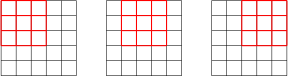
We can map apply_kernel() across the coordinate grid. That is, we'll be taking our 3×3 kernel, and applying it to each 3×3 section of our image. For instance, <<nopad_conv>> shows the positions a 3×3 kernel can be applied to in the first row of a 5×5 image.
我们可以在坐标网格上映射apply_kernel()。也就是说,我们将获取3×3卷积核,并将其应用于图像的每个3×3部分。例如,<<nopad_conv>>显示了5×5图像的第一行中可以应用3×3卷积核的位置。
To get a grid of coordinates we can use a nested list comprehension, like so:
要获得坐标网格,我们可以使用嵌套列表推导式,如下所示:
[[(i,j) for j in range(1,5)] for i in range(1,5)]Output
[[(1, 1), (1, 2), (1, 3), (1, 4)],
 [(2, 1), (2, 2), (2, 3), (2, 4)],
 [(3, 1), (3, 2), (3, 3), (3, 4)],
 [(4, 1), (4, 2), (4, 3), (4, 4)]]
note: Nested List Comprehensions: Nested list comprehensions are used a lot in Python, so if you haven't seen them before, take a few minutes to make sure you understand what's happening here, and experiment with writing your own nested list comprehensions.
注意:嵌套列表推导式:嵌套列表推导式在Python中被大量使用,因此如果您以前没有见过它们,请花几分钟时间确保您了解这里发生的事情,并尝试编写自己的嵌套列表推导式。
Here's the result of applying our kernel over a coordinate grid:
下面是在坐标网格上应用卷积核的结果:
rng = range(1,27)
top_edge3 = tensor([[apply_kernel(i,j,top_edge) for j in rng] for i in rng])

show_image(top_edge3);
Output
<Figure size 72x72 with 1 Axes>

Looking good! Our top edges are black, and bottom edges are white (since they are the opposite of top edges). Now that our image contains negative numbers too, matplotlib has automatically changed our colors so that white is the smallest number in the image, black the highest, and zeros appear as gray.
We can try the same thing for left edges:
看起来不错!我们的上边缘是黑色的,下边缘是白色的(因为它们与上边缘相反)。现在我们的图像也包含负数,matplotlib自动更改了颜色,使白色是图像中最小的数字,黑色是最大的数字,0显示为灰色。
我们可以对左边缘进行相同的操作:
left_edge = tensor([[-1,1,0],
                    [-1,1,0],
                    [-1,1,0]]).float()

left_edge3 = tensor([[apply_kernel(i,j,left_edge) for j in rng] for i in rng])

show_image(left_edge3);
Output
<Figure size 72x72 with 1 Axes>

As we mentioned before, a convolution is the operation of applying such a kernel over a grid in this way. In the paper "A Guide to Convolution Arithmetic for Deep Learning" there are many great diagrams showing how image kernels can be applied. Here's an example from the paper showing (at the bottom) a light blue 4×4 image, with a dark blue 3×3 kernel being applied, creating a 2×2 green output activation map at the top.
正如我们之前提到的,卷积就是以这种方式在网格上应用这样一个卷积核的操作。在“深度学习卷积算法指南”一文中,有许多很棒的图表展示了如何应用图像核。下面是本文中的一个示例,显示了一个浅蓝色的4×4图像(在底部),应用了一个深蓝色的3×3内核,并在顶部创建了一个2×2绿色的输出激活映射。
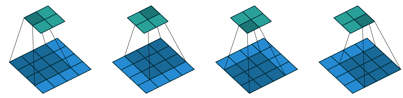
Look at the shape of the result. If the original image has a height of h and a width of w, how many 3×3 windows can we find? As you can see from the example, there are h-2 by w-2 windows, so the image we get has a result as a height of h-2 and a width of w-2.
看看结果的形状。如果原始图像的高度为h,宽度为w,我们可以找到多少个3×3窗口?从示例中可以看出,有h-2×w-2个窗口,因此我们得到的图像的高度为h-2,宽度为w-2。
We won't implement this convolution function from scratch, but use PyTorch's implementation instead (it is way faster than anything we could do in Python).
我们不会从头开始实现这个卷积函数,而是使用PyTorch的实现(它比我们用Python做的任何事情都要快得多)。
Convolutions in PyTorch
PyTorch中的卷积
Convolution is such an important and widely used operation that PyTorch has it built in. It's called F.conv2d (recall that F is a fastai import from torch.nn.functional, as recommended by PyTorch). The PyTorch docs tell us that it includes these parameters:
- input:: input tensor of shape
(minibatch, in_channels, iH, iW) - weight:: filters of shape
(out_channels, in_channels, kH, kW)
Here iH,iW is the height and width of the image (i.e., 28,28), and kH,kW is the height and width of our kernel (3,3). But apparently PyTorch is expecting rank-4 tensors for both these arguments, whereas currently we only have rank-2 tensors (i.e., matrices, or arrays with two axes).
The reason for these extra axes is that PyTorch has a few tricks up its sleeve. The first trick is that PyTorch can apply a convolution to multiple images at the same time. That means we can call it on every item in a batch at once!
The second trick is that PyTorch can apply multiple kernels at the same time. So let's create the diagonal-edge kernels too, and then stack all four of our edge kernels into a single tensor:
卷积是一个很重要且广泛使用的操作,PyTorch内置了它。它被称为F.conv2d(回想一下,F是从torch.nn.functional中的一个fastai导入,正如PyTorch推荐的那样)。PyTorch文档告诉我们它包含以下参数:
- 输入:: 输入张量的形状
(minibatch, in_channels, iH, iW) - 权重:: 过滤器的形状
(out_channels, in_channels, kH, kW)
这里iH,iW是图像的高度和宽度(即28,28),而kH,kW是我们卷积核的高度和宽度(3,3)。但显然PyTorch对这两个参数都期望4阶的张量,而目前我们只有2阶的张量(即具有两个轴的矩阵或数组)。
这些额外轴的原因是PyTorch有一些锦囊妙计。第一个技巧是PyTorch可以同时对多个图像进行卷积操作。这意味着我们可以一次调用批处理中的每个项目!
第二个技巧是PyTorch可以同时应用多个卷积核。因此,让我们也创建对角线边缘核,然后将所有四个边缘卷积核堆叠成一个张量:
diag1_edge = tensor([[ 0,-1, 1],
                     [-1, 1, 0],
                     [ 1, 0, 0]]).float()
diag2_edge = tensor([[ 1,-1, 0],
                     [ 0, 1,-1],
                     [ 0, 0, 1]]).float()

edge_kernels = torch.stack([left_edge, top_edge, diag1_edge, diag2_edge])
edge_kernels.shape
Output
torch.Size([4, 3, 3])
To test this, we'll need a DataLoader and a sample mini-batch. Let's use the data block API:
为了测试这一点,我们需要一个DataLoader和一个样本小批量。让我们使用数据块API:
mnist = DataBlock((ImageBlock(cls=PILImageBW), CategoryBlock),
                  get_items=get_image_files,
                  splitter=GrandparentSplitter(),
                  get_y=parent_label)

dls = mnist.dataloaders(path)
xb,yb = first(dls.valid)
xb.shape
Output
torch.Size([64, 1, 28, 28])
By default, fastai puts data on the GPU when using data blocks. Let's move it to the CPU for our examples:
默认情况下,fastai在使用数据块时会将数据放在GPU上。让我们将其移动到CPU上进行示例:
xb,yb = to_cpu(xb),to_cpu(yb)One batch contains 64 images, each of 1 channel, with 28×28 pixels. F.conv2d can handle multichannel (i.e., color) images too. A channel is a single basic color in an image—for regular full-color images there are three channels, red, green, and blue. PyTorch represents an image as a rank-3 tensor, with dimensions [channels, rows, columns].
We'll see how to handle more than one channel later in this chapter. Kernels passed to F.conv2d need to be rank-4 tensors: [channels_in, features_out, rows, columns]. edge_kernels is currently missing one of these. We need to tell PyTorch that the number of input channels in the kernel is one, which we can do by inserting an axis of size one (this is known as a unit axis) in the first location, where the PyTorch docs show in_channels is expected. To insert a unit axis into a tensor, we use the unsqueeze method:
一个批次包含64张图像,每张图像有1个通道,像素大小为28×28。F.conv2d也可以处理多通道(即彩色)图像。通道是图像中的单一基本颜色——对于常规的全彩色图像,有三个通道,红色、绿色和蓝色。PyTorch将图像表示为秩为3的张量,维度为[channels, rows, columns]。
我们将在本章后面看到如何处理多个通道。传递给F.conv2d的卷积核需要是4阶的张量:[channels_in, features_out, rows, columns]。edge_kernels目前缺少其中一个。我们需要告诉PyTorch卷积核中的输入通道数为1,我们可以通过在第一个位置插入一个大小为1的轴(这称为单位轴)来实现,PyTorch文档期望在这个位置显示in_channels。为了在张量中插入一个单位轴,我们使用unsqueeze方法:
edge_kernels.shape,edge_kernels.unsqueeze(1).shapeOutput
(torch.Size([4, 3, 3]), torch.Size([4, 1, 3, 3]))
This is now the correct shape for edge_kernels. Let's pass this all to conv2d:
现在这是edge_kernels的正确形状。让我们将其全部传递给conv2d:
edge_kernels = edge_kernels.unsqueeze(1)batch_features = F.conv2d(xb, edge_kernels)
batch_features.shapeOutput
torch.Size([64, 4, 26, 26])
The output shape shows we gave 64 images in the mini-batch, 4 kernels, and 26×26 edge maps (we started with 28×28 images, but lost one pixel from each side as discussed earlier). We can see we get the same results as when we did this manually:
输出形状显示我们在小批处理中给出了64张图像、4个卷积核和26×26个边缘映射(我们从28×28图像开始,但如前所述,每边损失了一个像素)。我们可以看到,我们得到了与手动操作相同的结果:
show_image(batch_features[0,0]);Output
<Figure size 72x72 with 1 Axes>

The most important trick that PyTorch has up its sleeve is that it can use the GPU to do all this work in parallel—that is, applying multiple kernels, to multiple images, across multiple channels. Doing lots of work in parallel is critical to getting GPUs to work efficiently; if we did each of these operations one at a time, we'd often run hundreds of times slower (and if we used our manual convolution loop from the previous section, we'd be millions of times slower!). Therefore, to become a strong deep learning practitioner, one skill to practice is giving your GPU plenty of work to do at a time.
PyTorch拥有的最重要的技巧是它可以使用GPU并行完成所有这些工作——也就是说,通过多个通道将多个卷积核应用于多个图像。并行地完成大量的工作对GPU高效工作至关重要;如果我们一次一个地完成这些操作,我们的运行速度通常会慢数百倍(如果我们使用上一节中的手动卷积循环,我们的运行速度会慢数百万倍!)因此,要成为一个强大的深度学习实践者,一个需要练习的技能就是让你的GPU一次做大量的工作。
It would be nice to not lose those two pixels on each axis. The way we do that is to add padding, which is simply additional pixels added around the outside of our image. Most commonly, pixels of zeros are added.
最好不要丢失每个轴上的这两个像素。我们这样做的方法是添加填充,这只是在图像外部添加的额外像素。最常见的是添加零像素。
Strides and Padding
步幅和填充
With appropriate padding, we can ensure that the output activation map is the same size as the original image, which can make things a lot simpler when we construct our architectures. <<pad_conv>> shows how adding padding allows us to apply the kernels in the image corners.
通过适当的填充,我们可以确保输出的激活映射与原始图像的大小相同,这可以使我们构建架构时的事情简单很多。<<pad_conv>>显示了添加填充操作是如何允许我们在图像角应用卷积核的。

With a 5×5 input, 4×4 kernel, and 2 pixels of padding, we end up with a 6×6 activation map, as we can see in <<four_by_five_conv>>.
使用5×5输入、4×4卷积核和2像素填充,我们最终得到6×6激活映射,正如我们在<<four_by_five_conv>>中看到的那样。
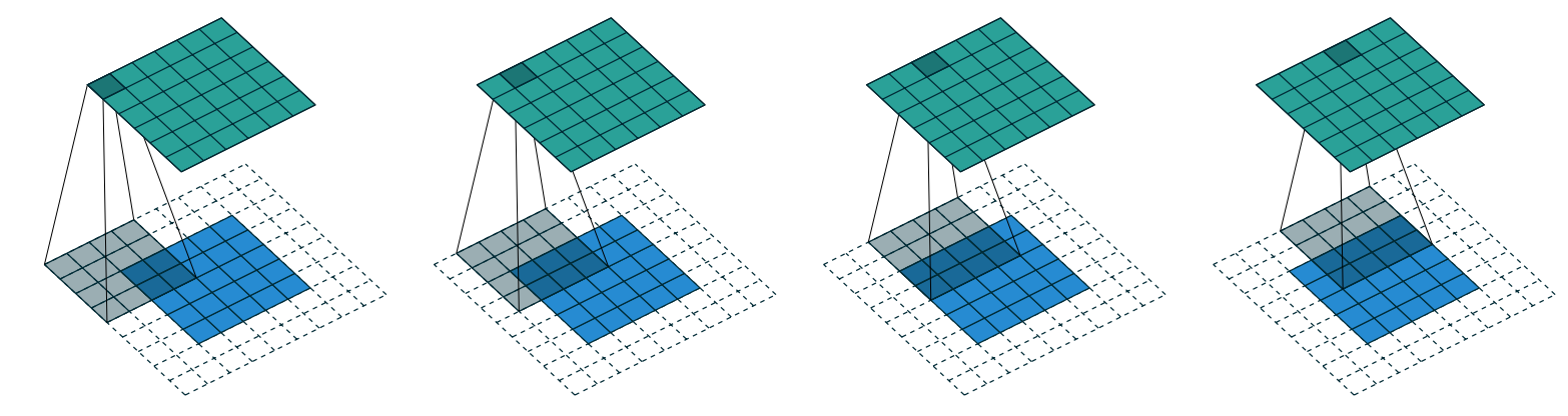
If we add a kernel of size ks by ks (with ks an odd number), the necessary padding on each side to keep the same shape is ks//2. An even number for ks would require a different amount of padding on the top/bottom and left/right, but in practice we almost never use an even filter size.
So far, when we have applied the kernel to the grid, we have moved it one pixel over at a time. But we can jump further; for instance, we could move over two pixels after each kernel application, as in <<three_by_five_conv>>. This is known as a stride-2 convolution. The most common kernel size in practice is 3×3, and the most common padding is 1. As you'll see, stride-2 convolutions are useful for decreasing the size of our outputs, and stride-1 convolutions are useful for adding layers without changing the output size.
如果我们添加一个大小为ks×ks的内核(其中ks是奇数),则每边保持相同形状所需的填充是ks//2。偶数的ks将需要不同数量的上/下和左/右填充,但在实践中,我们几乎从不使用偶数的过滤器大小。
到目前为止,当我们将卷积核应用到网格中时,每次移动一个像素。但我们可以跳得更远;例如,我们可以在每次卷积核应用后移动两个像素,如<<three_by_five_conv>>。这被称为stride-2卷积。实践中最常见的卷积核大小是3×3,最常见的填充是1。正如您将看到的,stride-2卷积对于减小输出大小很有用,而stride-1卷积对于在不改变输出大小的情况下添加图层很有用。
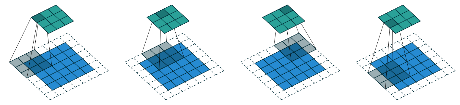
In an image of size h by w, using a padding of 1 and a stride of 2 will give us a result of size (h+1)//2 by (w+1)//2. The general formula for each dimension is (n + 2*pad - ks)//stride + 1, where pad is the padding, ks, the size of our kernel, and stride is the stride.
在大小为h×w的图像中,使用1的填充和2的步幅将得到大小为(h+1)//2×(w+1)//2的结果。每个维度的一般公式是(n + 2*pad - ks)//stride + 1,其中pad是填充,ks是卷积核的大小,stride是步幅。
Let's now take a look at how the pixel values of the result of our convolutions are computed.
现在让我们看一下卷积结果的像素值是如何计算的。
Understanding the Convolution Equations
###了解卷积方程
To explain the math behind convolutions, fast.ai student Matt Kleinsmith came up with the very clever idea of showing CNNs from different viewpoints. In fact, it's so clever, and so helpful, we're going to show it here too!
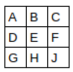
Here's our 3×3 pixel image, with each pixel labeled with a letter:
为了解释卷积背后的数学原理,fast.ai学生Matt Kleinsmith想出了一个非常聪明的主意从不同的角度展示CNNs。事实上,这非常聪明,非常有帮助,我们也将在这里展示它!
这是我们的3×3像素图像,每个像素都用字母标记:
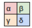
And here's our kernel, with each weight labeled with a Greek letter:
这是我们的卷积核,每个权重都标有一个希腊字母:
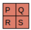
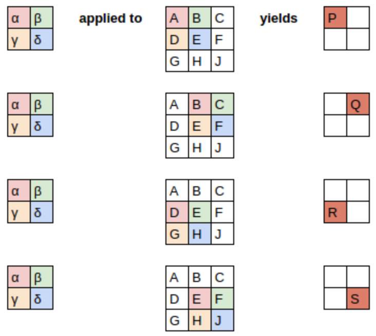
Since the filter fits in the image four times, we have four results:
由于过滤器在图像中拟合了四次,我们有四个结果:
<<apply_kernel>> shows how we applied the kernel to each section of the image to yield each result.
<<apply_kernel>>显示了我们如何将卷积核应用于图像的每个部分以产生每个结果。
The equation view is in <<eq_view>>.
方程视图在<<eq_view>>中。
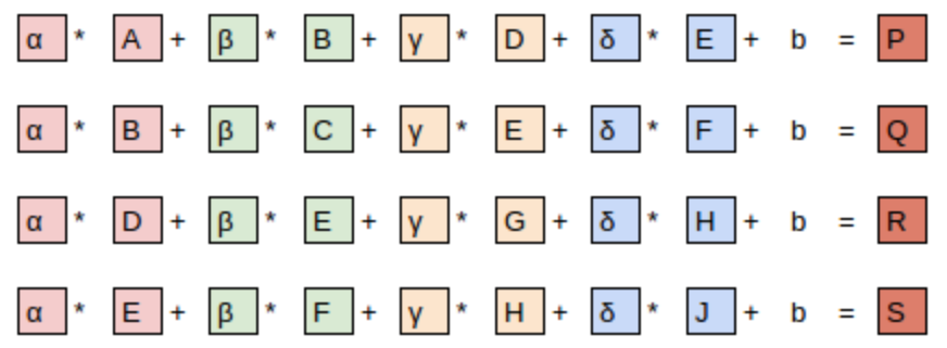
Notice that the bias term, b, is the same for each section of the image. You can consider the bias as part of the filter, just like the weights (α, β, γ, δ) are part of the filter.
请注意,偏置项b对于图像的每个部分都是相同的。您可以将偏置视为过滤器的一部分,就像权重 (α, β, γ, δ) 是过滤器的一部分一样。
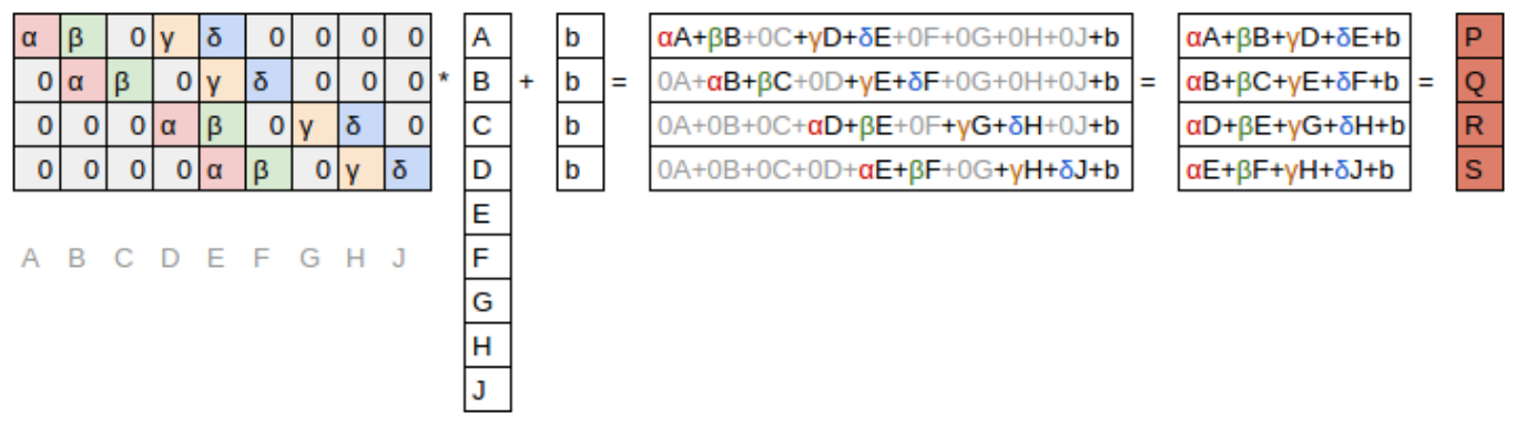
Here's an interesting insight—a convolution can be represented as a special kind of matrix multiplication, as illustrated in <<conv_matmul>>. The weight matrix is just like the ones from traditional neural networks. However, this weight matrix has two special properties:
- The zeros shown in gray are untrainable. This means that they’ll stay zero throughout the optimization process.
- Some of the weights are equal, and while they are trainable (i.e., changeable), they must remain equal. These are called shared weights.
The zeros correspond to the pixels that the filter can't touch. Each row of the weight matrix corresponds to one application of the filter.
这里有一个有趣的见解——卷积可以表示为一种特殊的矩阵乘法,如<<conv_matmul>>所示。权重矩阵与传统神经网络的权重矩阵相同。然而,这个权重矩阵有两个特殊的性质:
- 灰色显示的零是不可训练的。这意味着它们将在整个优化过程中保持为零。
- 有些权重是相等的,虽然它们是可训练的(即可变的),但它们必须保持相等。这些被称为共享权重。
零对应于过滤器不能触及的像素。权重矩阵的每一行对应于过滤器的一个应用。
Now that we understand what a convolution is, let's use them to build a neural net.
现在我们了解了什么是卷积,让我们使用它们来构建神经网络。
Our First Convolutional Neural Network
我们的第一个卷积神经网络
There is no reason to believe that some particular edge filters are the most useful kernels for image recognition. Furthermore, we've seen that in later layers convolutional kernels become complex transformations of features from lower levels, but we don't have a good idea of how to manually construct these.
Instead, it would be best to learn the values of the kernels. We already know how to do this—SGD! In effect, the model will learn the features that are useful for classification.
When we use convolutions instead of (or in addition to) regular linear layers we create a convolutional neural network (CNN).
没有理由相信某些特定的边缘过滤器是图像识别中最有用的核。此外,我们已经看到,在后面的层中,卷积核从较低层次变成了复杂的特征转换,但我们不知道如何手动构建这些。
相反,最好学习核的值。我们已经知道如何做到这一点——SGD!实际上,模型将学习对分类有用的特征。
当我们使用卷积而不是(或除了)常规线性层时,我们创建了一个卷积神经网络(CNN)。
Creating the CNN
创建CNN
Let's go back to the basic neural network we had in <<chapter_mnist_basics>>. It was defined like this:
让我们回到<<chapter_mnist_basics>>中的基本神经网络。它是这样定义的:
simple_net = nn.Sequential(
    nn.Linear(28*28,30),
    nn.ReLU(),
    nn.Linear(30,1)
)
We can view a model's definition:
我们可以查看模型的定义:
simple_netOutput
Sequential(
  (0): Linear(in_features=784, out_features=30, bias=True)
  (1): ReLU()
  (2): Linear(in_features=30, out_features=1, bias=True)
)
We now want to create a similar architecture to this linear model, but using convolutional layers instead of linear. nn.Conv2d is the module equivalent of F.conv2d. It's more convenient than F.conv2d when creating an architecture, because it creates the weight matrix for us automatically when we instantiate it.
Here's a possible architecture:
现在我们想创建一个类似于这个线性模型的架构,但是使用卷积层而不是线性层。nn.Conv2d是F.conv2d的等效的模块。在创建架构时,它比F.conv2d更方便,因为当我们实例化它时,它会自动为我们创建权重矩阵。
下面是一个可能的架构:
broken_cnn = sequential(
    nn.Conv2d(1,30, kernel_size=3, padding=1),
    nn.ReLU(),
    nn.Conv2d(30,1, kernel_size=3, padding=1)
)
One thing to note here is that we didn't need to specify 28×28 as the input size. That's because a linear layer needs a weight in the weight matrix for every pixel, so it needs to know how many pixels there are, but a convolution is applied over each pixel automatically. The weights only depend on the number of input and output channels and the kernel size, as we saw in the previous section.
Think about what the output shape is going to be, then let's try it and see:
这里需要注意的一点是,我们不需要指定28×28作为输入大小。这是因为线性层需要在权重矩阵中为每个像素设置一个权重,所以它需要知道有多少像素,但是卷积是自动施加在每个像素上的。正如我们在上一节中看到的,权重只取决于输入和输出通道的数量以及卷积核大小。
想想输出形状将是什么,然后让我们试试看:
broken_cnn(xb).shapeOutput
torch.Size([64, 1, 28, 28])
This is not something we can use to do classification, since we need a single output activation per image, not a 28×28 map of activations. One way to deal with this is to use enough stride-2 convolutions such that the final layer is size 1. That is, after one stride-2 convolution the size will be 14×14, after two it will be 7×7, then 4×4, 2×2, and finally size 1.
Let's try that now. First, we'll define a function with the basic parameters we'll use in each convolution:
这不是我们可以用来进行分类的东西,因为我们需要为每个图片提供一个输出激活,而不是一个28×28的激活映射。解决这个问题的一种方法是使用足够的stride-2卷积,使最终层的大小为1。也就是说,在一次stride-2卷积之后,大小将为14×14,两次之后将为7×7,然后是4×4、2×2,最后是大小为1。
现在让我们试试。首先,我们将定义一个函数,其基本参数将在每次卷积中使用:
def conv(ni, nf, ks=3, act=True):
    res = nn.Conv2d(ni, nf, stride=2, kernel_size=ks, padding=ks//2)
    if act: res = nn.Sequential(res, nn.ReLU())
    return res
important: Refactoring: Refactoring parts of your neural networks like this makes it much less likely you'll get errors due to inconsistencies in your architectures, and makes it more obvious to the reader which parts of your layers are actually changing.
重要:重构:像这样重构神经网络的一部分可以降低由于架构不一致而导致错误的可能性,并且让读者更清楚你的层的哪些部分实际上在变化。
When we use a stride-2 convolution, we often increase the number of features at the same time. This is because we're decreasing the number of activations in the activation map by a factor of 4; we don't want to decrease the capacity of a layer by too much at a time.
当我们使用stride-2卷积时,我们通常会同时增加特征的数量。这是因为我们将激活图中的激活数减少了4倍;我们不想一次过多地减少一层的容量。
jargon: channels and features: These two terms are largely used interchangeably, and refer to the size of the second axis of a weight matrix, which is, the number of activations per grid cell after a convolution. Features is never used to refer to the input data, but channels can refer to either the input data (generally channels are colors) or activations inside the network.
术语:通道和特征:这两个术语在很大程度上可以互换使用,它们指的是权重矩阵第二轴的大小,即卷积后每个网格单元的激活数。特征从不用于指代输入数据,但通道可以指代输入数据(通常通道是颜色)或网络内部的激活。
Here is how we can build a simple CNN:
以下是我们如何构建一个简单的CNN:
simple_cnn = sequential(
    conv(1 ,4),            #14x14
    conv(4 ,8),            #7x7
    conv(8 ,16),           #4x4
    conv(16,32),           #2x2
    conv(32,2, act=False), #1x1
    Flatten(),
)
j: I like to add comments like the ones here after each convolution to show how large the activation map will be after each layer. These comments assume that the input size is 28*28
j:我喜欢在每一层卷积之后添加像这里这样的注释,以显示每一层卷积之后激活图的大小。这些注释假设输入大小为28*28
Now the network outputs two activations, which map to the two possible levels in our labels:
现在网络输出两个激活,它们对应于我们的标签中两个可能的级别:
simple_cnn(xb).shapeOutput
torch.Size([64, 2])
We can now create our Learner:
我们现在可以创建我们的Learner:
learn = Learner(dls, simple_cnn, loss_func=F.cross_entropy, metrics=accuracy)To see exactly what's going on in the model, we can use summary:
要准确查看模型中发生的事情,我们可以使用summary:
learn.summary()Output
Sequential (Input shape: ['64 x 1 x 28 x 28'])
================================================================
Layer (type)         Output Shape         Param #    Trainable
================================================================
Conv2d               64 x 4 x 14 x 14     40         True
________________________________________________________________
ReLU                 64 x 4 x 14 x 14     0          False
________________________________________________________________
Conv2d               64 x 8 x 7 x 7       296        True
________________________________________________________________
ReLU                 64 x 8 x 7 x 7       0          False
________________________________________________________________
Conv2d               64 x 16 x 4 x 4      1,168      True
________________________________________________________________
ReLU                 64 x 16 x 4 x 4      0          False
________________________________________________________________
Conv2d               64 x 32 x 2 x 2      4,640      True
________________________________________________________________
ReLU                 64 x 32 x 2 x 2      0          False
________________________________________________________________
Conv2d               64 x 2 x 1 x 1       578        True
________________________________________________________________
Flatten              64 x 2               0          False
________________________________________________________________

Total params: 6,722
Total trainable params: 6,722
Total non-trainable params: 0

Optimizer used: <function Adam at 0x7fbc9c258cb0>
Loss function: <function cross_entropy at 0x7fbca9ba0170>

Callbacks:
  - TrainEvalCallback
  - Recorder
  - ProgressCallback
Note that the output of the final Conv2d layer is 64x2x1x1. We need to remove those extra 1x1 axes; that's what Flatten does. It's basically the same as PyTorch's squeeze method, but as a module.
Let's see if this trains! Since this is a deeper network than we've built from scratch before, we'll use a lower learning rate and more epochs:
请注意,最终的Conv2d层的输出是64x2x1x1。我们需要去除这些额外的1x1轴;这就是Flatten的作用。它基本上与PyTorch的squeeze方法相同,但它是作为一个模块。
让我们来看看这是否能起作用! 由于这是一个比我们以前从头开始建立的更深的网络,我们将使用较低的学习率和更多的训练轮数。
learn.fit_one_cycle(2, 0.01)Output
<IPython.core.display.HTML object>
| epoch | train_loss | valid_loss | accuracy | time |
|---|---|---|---|---|
| 0 | 0.072684 | 0.045110 | 0.990186 | 00:05 |
| 1 | 0.022580 | 0.030775 | 0.990186 | 00:05 |
Success! It's getting closer to the resnet18 result we had, although it's not quite there yet, and it's taking more epochs, and we're needing to use a lower learning rate. We still have a few more tricks to learn, but we're getting closer and closer to being able to create a modern CNN from scratch.
成功了!它越来越接近resnet18的结果了,尽管它还没有完成,而且需要更多的时间,我们需要使用更低的学习率。我们还有更多的技巧要学习,但我们离从零开始创建一个现代CNN越来越近了。
Understanding Convolution Arithmetic
了解卷积算法
We can see from the summary that we have an input of size 64x1x28x28. The axes are batch,channel,height,width. This is often represented as NCHW (where N refers to batch size). Tensorflow, on the other hand, uses NHWC axis order. The first layer is:
从摘要中我们可以看到,我们有一个大小为64x1x28x28的输入。轴是batch,channel,height,width。这通常表示为NCHW(其中N表示批量大小)。另一方面,Tensorflow使用NHWC轴序。第一层是:
m = learn.model[0]
m
Output
Sequential(
  (0): Conv2d(1, 4, kernel_size=(3, 3), stride=(2, 2), padding=(1, 1))
  (1): ReLU()
)
So we have 1 input channel, 4 output channels, and a 3×3 kernel. Let's check the weights of the first convolution:
因此,我们有1个输入通道,4个输出通道和一个3×3卷积核。让我们检查第一个卷积的权重:
m[0].weight.shapeOutput
torch.Size([4, 1, 3, 3])
The summary shows we have 40 parameters, and 4*1*3*3 is 36. What are the other four parameters? Let's see what the bias contains:
总结显示我们有40个参数,4*1*3*3是36个。其他四个参数是什么?让我们看看偏差包含什么:
m[0].bias.shapeOutput
torch.Size([4])
We can now use this information to clarify our statement in the previous section: "When we use a stride-2 convolution, we often increase the number of features because we're decreasing the number of activations in the activation map by a factor of 4; we don't want to decrease the capacity of a layer by too much at a time."
There is one bias for each channel. (Sometimes channels are called features or filters when they are not input channels.) The output shape is 64x4x14x14, and this will therefore become the input shape to the next layer. The next layer, according to summary, has 296 parameters. Let's ignore the batch axis to keep things simple. So for each of 14*14=196 locations we are multiplying 296-8=288 weights (ignoring the bias for simplicity), so that's 196*288=56_448 multiplications at this layer. The next layer will have 7*7*(1168-16)=56_448 multiplications.
What happened here is that our stride-2 convolution halved the grid size from 14x14 to 7x7, and we doubled the number of filters from 8 to 16, resulting in no overall change in the amount of computation. If we left the number of channels the same in each stride-2 layer, the amount of computation being done in the net would get less and less as it gets deeper. But we know that the deeper layers have to compute semantically rich features (such as eyes or fur), so we wouldn't expect that doing less computation would make sense.
我们现在可以使用这些信息来澄清我们在上一节中的陈述:“当我们使用stride-2卷积时,我们通常会增加特征的数量,因为我们将激活图中的激活数量减少了4倍;我们不想一次减少太多一层的容量。”
每个通道都有一个偏置。(有时,当通道不是输入通道时,它们被称为特征或过滤器。)输出形状是64x4x14x14,因此这将成为下一层的输入形状。根据summary,下一层有296个参数。为了简单起见,我们忽略批处理轴。所以对于14*14=196的每个位置,我们要乘以296-8=288的权重(为了简单起见忽略偏置),所以这一层是196*288=56_448的乘法。下一层是7*7*(1168-16)=56_448的乘法。
这里发生的事情是,我们的stride-2卷积将网格大小从14x14减半到7x7,我们将过滤器数量从8个增加到16个,导致总体计算量没有变化。如果我们保持每个步幅为2的层的通道数量不变,那么随着网络越深,所做的计算量就会越来越少。但我们知道更深的层必须计算语义丰富的特征(例如眼睛或毛皮),因此我们不会期望进行更少的计算是有意义的。
Another way to think of this is based on receptive fields.
另一种思考方法是基于感受野。
Receptive Fields
感受野
The receptive field is the area of an image that is involved in the calculation of a layer. On the book's website, you'll find an Excel spreadsheet called conv-example.xlsx that shows the calculation of two stride-2 convolutional layers using an MNIST digit. Each layer has a single kernel. <> shows what we see if we click on one of the cells in the conv2 section, which shows the output of the second convolutional layer, and click trace precedents.
感受野是图像中涉及到层计算的区域。在这本书的网站上,您会找到一个名为conv-example.xlsx的Excel电子表格,它显示了使用MNIST数字计算两个stride-2卷积层的情况。每个层都有一个卷积核。<>显示了如果我们单击conv2部分中的一个单元格(该部分显示第二层卷积层的输出),然后单击跟踪先例时我们所看到的内容。
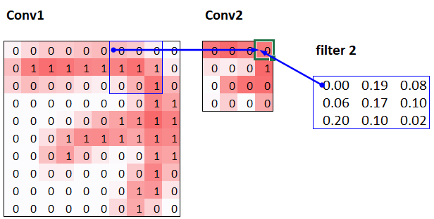
Here, the cell with the green border is the cell we clicked on, and the blue highlighted cells are its precedents—that is, the cells used to calculate its value. These cells are the corresponding 3×3 area of cells from the input layer (on the left), and the cells from the filter (on the right). Let's now click trace precedents again, to see what cells are used to calculate these inputs. <> shows what happens.
在这里,绿色边框的单元格是我们单击的单元格,蓝色突出显示的单元格是它的先例-即用于计算其值的单元格。这些单元格是来自输入层(左边)的单元格对应的3×3区域,以及来自过滤器(右边)的单元格。现在让我们再次单击跟踪先例,以查看使用哪些单元格来计算这些输入。<> 显示发生了什么。
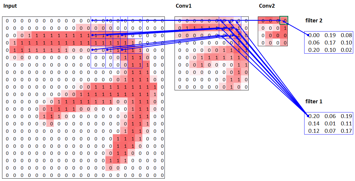
In this example, we have just two convolutional layers, each of stride 2, so this is now tracing right back to the input image. We can see that a 7×7 area of cells in the input layer is used to calculate the single green cell in the Conv2 layer. This 7×7 area is the receptive field in the input of the green activation in Conv2. We can also see that a second filter kernel is needed now, since we have two layers.
As you see from this example, the deeper we are in the network (specifically, the more stride-2 convs we have before a layer), the larger the receptive field for an activation in that layer. A large receptive field means that a large amount of the input image is used to calculate each activation in that layer is. We now know that in the deeper layers of the network we have semantically rich features, corresponding to larger receptive fields. Therefore, we'd expect that we'd need more weights for each of our features to handle this increasing complexity. This is another way of saying the same thing we mentioned in the previous section: when we introduce a stride-2 conv in our network, we should also increase the number of channels.
在这个例子中,我们只有两个卷积层,每一个都是步幅为2,所以现在这是直接追踪到输入图像。我们可以看到输入层中的7×7区域的单元格用于计算Conv2层中的单个绿色单元格。这个7×7区域是Conv2中绿色激活输入中的感受野。我们还可以看到现在需要第二个过滤器卷积核,因为我们有两层。
正如你从这个例子中看到的,我们在网络中的深度越深(具体地说,我们在一层之前的stride-2卷积越多),该层中激活的感受野就越大。一个大的感受野意味着大量的输入图像用于计算该层中的每个激活。我们现在知道,在更深层次的网络中,我们拥有丰富的语义特征,与更大的感受野相对应。因此,我们需要为每个特征增加更多的权重来处理这种不断增加的复杂性。这是我们在上一节中提到的同一件事的另一种说法:当我们在网络中引入stride-2卷积时,我们也应该增加通道的数量。
When writing this particular chapter, we had a lot of questions we needed answers for, to be able to explain CNNs to you as best we could. Believe it or not, we found most of the answers on Twitter. We're going to take a quick break to talk to you about that now, before we move on to color images.
在写这一章的时候,我们有很多问题需要回答,以便能够尽我们所能向你解释CNN。信不信由你,我们在Twitter上找到了大部分答案。在我们继续讲彩色图像之前,我们先休息一下来谈谈这个问题。
A Note About Twitter
关于Twitter的注意事项
We are not, to say the least, big users of social networks in general. But our goal in writing this book is to help you become the best deep learning practitioner you can, and we would be remiss not to mention how important Twitter has been in our own deep learning journeys.
You see, there's another part of Twitter, far away from Donald Trump and the Kardashians, which is the part of Twitter where deep learning researchers and practitioners talk shop every day. As we were writing this section, Jeremy wanted to double-check that what we were saying about stride-2 convolutions was accurate, so he asked on Twitter:
至少可以说,我们不是社交网络的大用户。但我们写这本书的目标是帮助你成为最好的深度学习实践者,我们不应该忽视Twitter在我们自己的深度学习旅程中是多么重要。
你看,Twitter的另一个部分,远离Donald Trump和the Kardashians,这是深度学习研究者和从业者每天谈论的Twitter部分。当我们写这一部分的时候,Jeremy想仔细检查我们所说的stride-2卷积是否准确,所以他在Twitter上问道:

A few minutes later, this answer popped up:
几分钟后,答案出现了:
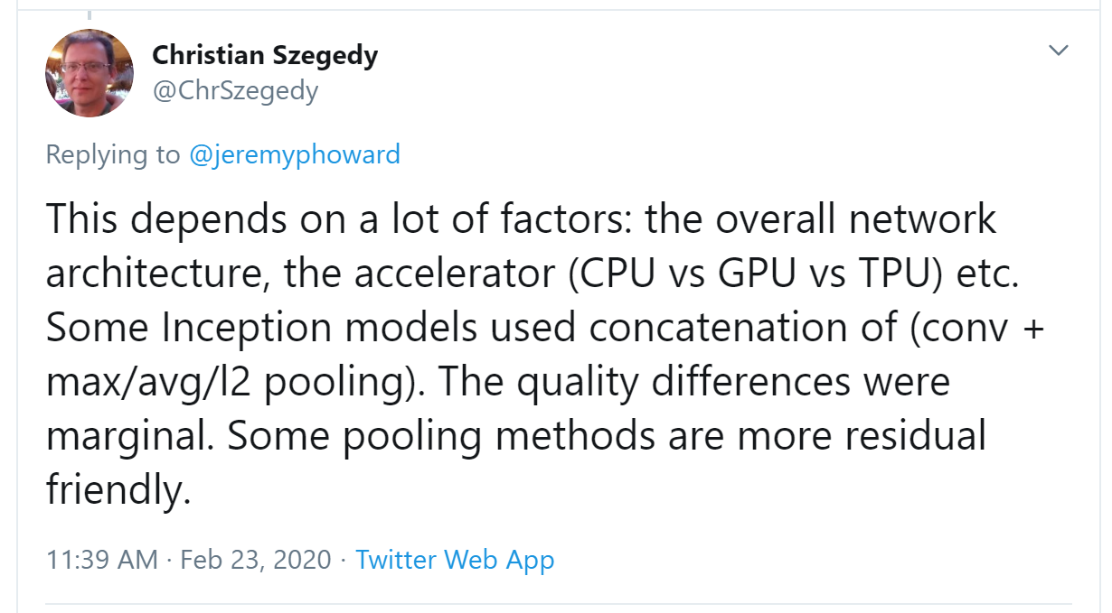
Christian Szegedy is the first author of Inception, the 2014 ImageNet winner and source of many key insights used in modern neural networks. Two hours later, this appeared:
Christian Szegedy是《Inception》的第一作者,该书是2014年ImageNet奖得主,是现代神经网络中许多关键见解的来源。两小时后,这出现了:
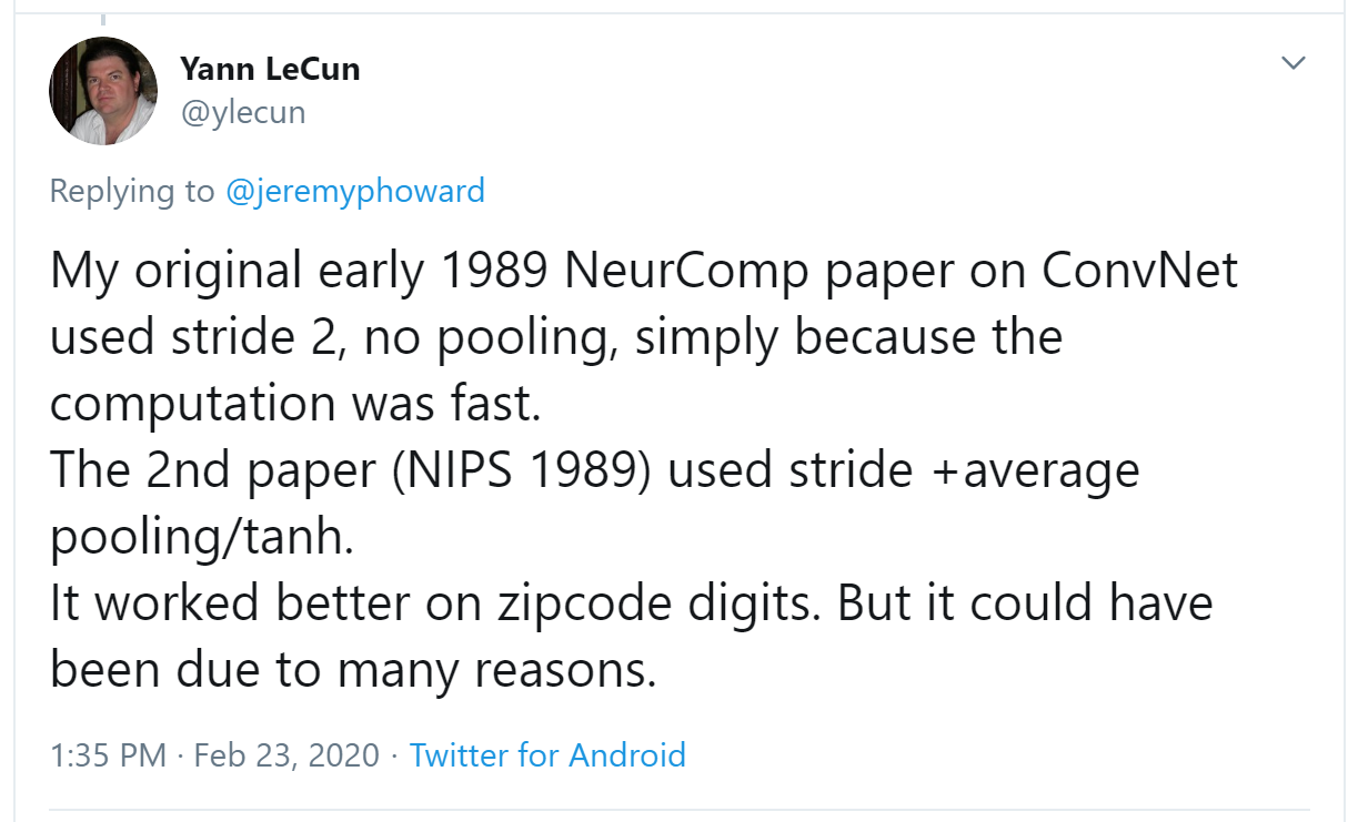
Do you recognize that name? You saw it in <<chapter_production>>, when we were talking about the Turing Award winners who established the foundations of deep learning today!
Jeremy also asked on Twitter for help checking our description of label smoothing in <<chapter_sizing_and_tta>> was accurate, and got a response again from directly from Christian Szegedy (label smoothing was originally introduced in the Inception paper):
你认识这个名字吗?你在<<chapter_production>>中看到过,当我们谈论为今天的深度学习奠定基础的图灵奖获得者时!
Jeremy还在Twitter上请求帮助检查我们对<<chapter_sizing_and_tta>>中标签平滑的描述是否准确,并直接得到了Christian Szegedy的再次回应(标签平滑最初是在《Inception》论文中引入的):

Many of the top people in deep learning today are Twitter regulars, and are very open about interacting with the wider community. One good way to get started is to look at a list of Jeremy's recent Twitter likes, or Sylvain's. That way, you can see a list of Twitter users that we think have interesting and useful things to say.
Twitter is the main way we both stay up to date with interesting papers, software releases, and other deep learning news. For making connections with the deep learning community, we recommend getting involved both in the fast.ai forums and on Twitter.
如今,许多深度学习领域的顶尖人士都是Twitter的常客,并且对与更广泛的社区互动非常开放。一个好的开始方法是查看Jeremy最近在Twitter上点赞的列表或Sylvan的。这样,你就可以看到一个Twitter用户列表,我们认为这些用户所说的内容是有趣并且有用的。
Twitter是我们了解最新有趣的论文、软件发布和其他深度学习新闻的主要途径。为了与深度学习社区建立联系,我们建议同时参与fast.ai论坛和Twitter。
That said, let's get back to the meat of this chapter. Up until now, we have only shown you examples of pictures in black and white, with one value per pixel. In practice, most colored images have three values per pixel to define their color. We'll look at working with color images next.
也就是说,让我们回到本章的重点。到目前为止,我们只展示了一些黑白图片的例子,每个像素有一个值。实际上,大多数彩色图像每个像素有三个值来定义它们的颜色。接下来我们将讨论如何处理彩色图像。
`# This is formatted as code`Color Images
彩色图像
A colour picture is a rank-3 tensor:
彩色图片是3阶张量:
im = image2tensor(Image.open(image_bear()))
im.shape
Output
torch.Size([3, 1000, 846])
show_image(im);Output
<Figure size 360x360 with 1 Axes>
[省略较大 image/png 输出]
The first axis contains the channels, red, green, and blue:
第一个轴包含通道,红色、绿色和蓝色:
_,axs = subplots(1,3)
for bear,ax,color in zip(im,axs,('Reds','Greens','Blues')):
    show_image(255-bear, ax=ax, cmap=color)
Output
<Figure size 864x288 with 3 Axes>
[省略较大 image/png 输出]
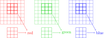
We saw what the convolution operation was for one filter on one channel of the image (our examples were done on a square). A convolutional layer will take an image with a certain number of channels (three for the first layer for regular RGB color images) and output an image with a different number of channels. Like our hidden size that represented the numbers of neurons in a linear layer, we can decide to have as many filters as we want, and each of them will be able to specialize, some to detect horizontal edges, others to detect vertical edges and so forth, to give something like we studied in <<chapter_production>>.
In one sliding window, we have a certain number of channels and we need as many filters (we don't use the same kernel for all the channels). So our kernel doesn't have a size of 3 by 3, but ch_in (for channels in) is 3 by 3. On each channel, we multiply the elements of our window by the elements of the coresponding filter, then sum the results (as we saw before) and sum over all the filters. In the example given in <>, the result of our conv layer on that window is red + green + blue.
我们看到了图像的一个通道上的一个过滤器的卷积运算(我们的例子是在一个正方形上做的)。卷积层将获取具有一定通道数的图像(第一层为3个通道,用于常规RGB彩色图像),并输出具有不同通道数的图像。就像我们表示线性层中神经元数量的隐藏大小一样,我们可以决定有多少过滤器,并且每个过滤器都可以专业化,一些用来检测水平边缘,另一些用来检测垂直边缘,等等,来给出我们在<<chapter_production>中研究的东西。
在一个滑动窗口中,我们有一定数量的通道,我们需要尽可能多的过滤器(我们不会对所有通道使用相同的卷积核)。所以我们的卷积核的大小不是3×3,但是ch_in(对于通道)是3×3。在每个通道上,我们将窗口的元素与相应过滤器的元素相乘,然后将结果求和(正如我们之前看到的)并对所有过滤器求和。在<>中给出的例子中,我们在该窗口上的卷积层的结果是红色+绿色+蓝色。
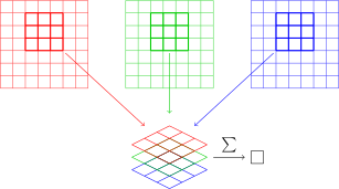
So, in order to apply a convolution to a color picture we require a kernel tensor with a size that matches the first axis. At each location, the corresponding parts of the kernel and the image patch are multiplied together.
These are then all added together, to produce a single number, for each grid location, for each output feature, as shown in <>.
因此,为了将卷积应用于彩色图片,我们需要一个大小与第一轴匹配的卷积核张量。在每个位置,卷积核和图像块的相应部分相乘在一起。
然后将这些全部相加在一起,为每个网格位置和每个输出特征生成一个数字,如<>所示。
Then we have ch_out filters like this, so in the end, the result of our convolutional layer will be a batch of images with ch_out channels and a height and width given by the formula outlined earlier. This give us ch_out tensors of size ch_in x ks x ks that we represent in one big tensor of four dimensions. In PyTorch, the order of the dimensions for those weights is ch_out x ch_in x ks x ks.
Additionally, we may want to have a bias for each filter. In the preceding example, the final result for our convolutional layer would be in that case. Like in a linear layer, there are as many bias as we have kernels, so the biases is a vector of size ch_out.
There are no special mechanisms required when setting up a CNN for training with color images. Just make sure your first layer has three inputs.
There are lots of ways of processing color images. For instance, you can change them to black and white, change from RGB to HSV (hue, saturation, and value) color space, and so forth. In general, it turns out experimentally that changing the encoding of colors won't make any difference to your model results, as long as you don't lose information in the transformation. So, transforming to black and white is a bad idea, since it removes the color information entirely (and this can be critical; for instance, a pet breed may have a distinctive color); but converting to HSV generally won't make any difference.
Now you know what those pictures in <<chapter_intro>> of "what a neural net learns" from the Zeiler and Fergus paper mean! This is their picture of some of the layer 1 weights which we showed:
然后我们有这样的ch_out过滤器,所以最后,我们卷积层的结果将是一批具有ch_out通道的图像,高度和宽度由前面概述的公式给出。这给了我们ch_out大小的张量ch_in x ks x ks,我们用一个四维的大张量来表示。在PyTorch中,这些权重的维度顺序是ch_out x ch_in x ks x ks。
此外,我们可能希望每个过滤器都有一个偏置。在前面的例子中,卷积层的最终结果将是。就像在线性层中,我们有多少卷积核就有多少偏置,所以偏置是一个大小为ch_out的向量。
在设置CNN进行彩色图像训练时,不需要特殊的机制。只要确保你的第一层有三个输入。
处理彩色图像的方法有很多。例如,你可以将它们更改为黑白图像,从RGB更改为HSV(色调、饱和度和值)颜色空间,等等。一般来说,实验证明,只要在转换过程中不丢失信息,改变颜色编码不会对模型结果产生任何影响。因此,转换为黑白图像是一个坏主意,因为它完全删除了颜色信息(这可能是至关重要的;例如,一个宠物品种可能有独特的颜色);但是转换为HSV通常不会有任何区别。
现在你知道<<chapter_intro>>中的那些来自Zeiler和Fergus论文中“神经网络学习”的图片的意思了!这是我们展示的一些他们的第一层权重的图片:
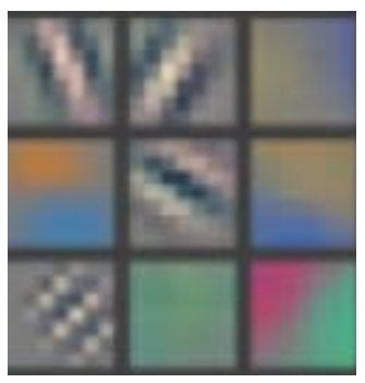
This is taking the three slices of the convolutional kernel, for each output feature, and displaying them as images. We can see that even though the creators of the neural net never explicitly created kernels to find edges, for instance, the neural net automatically discovered these features using SGD.
Now let's see how we can train these CNNs, and show you all the techniques fastai uses under the hood for efficient training.
这是对每个输出特征提取卷积核的三个切片,并将它们显示为图像。我们可以看到,即使神经网络的创建者从未明确地创建卷积核来寻找边缘,例如,神经网络使用SGD自动发现这些特征。
现在让我们看看如何训练这些CNN,并向你展示fastai用于高效训练的所有技术。
Improving Training Stability
提高训练稳定性
Since we are so good at recognizing 3s from 7s, let's move on to something harder—recognizing all 10 digits. That means we'll need to use MNIST instead of MNIST_SAMPLE:
既然我们非常擅长从7中识别3,让我们转向更难的东西——识别所有的10位数。这意味着我们需要使用MNIST而不是MNIST_SAMPLE:
path = untar_data(URLs.MNIST)#hide
Path.BASE_PATH = pathpath.ls()Output
(#2) [Path('testing'),Path('training')]The data is in two folders named training and testing, so we have to tell GrandparentSplitter about that (it defaults to train and valid). We did do that in the get_dls function, which we create to make it easy to change our batch size later:
数据位于名为training和testing的两个文件夹中,因此我们必须告诉GrandparentSplitter(默认为train和valid)。我们在get_dls函数中做到了这一点,我们创建这个函数是为了方便以后更改批处理大小:
def get_dls(bs=64):
    return DataBlock(
        blocks=(ImageBlock(cls=PILImageBW), CategoryBlock),
        get_items=get_image_files,
        splitter=GrandparentSplitter('training','testing'),
        get_y=parent_label,
        batch_tfms=Normalize()
    ).dataloaders(path, bs=bs)

dls = get_dls()
Remember, it's always a good idea to look at your data before you use it:
记住,在使用数据之前查看数据总是一个好主意:
dls.show_batch(max_n=9, figsize=(4,4))Output
<Figure size 288x288 with 9 Axes>

Now that we have our data ready, we can train a simple model on it.
现在我们已经准备好了数据,我们可以在上面训练一个简单的模型。
A Simple Baseline
一个简单的参照物
Earlier in this chapter, we built a model based on a conv function like this:
在本章的前面,我们构建了一个基于conv函数的模型,如下所示:
def conv(ni, nf, ks=3, act=True):
    res = nn.Conv2d(ni, nf, stride=2, kernel_size=ks, padding=ks//2)
    if act: res = nn.Sequential(res, nn.ReLU())
    return res
Let's start with a basic CNN as a baseline. We'll use the same one as earlier, but with one tweak: we'll use more activations. Since we have more numbers to differentiate, it's likely we will need to learn more filters.
As we discussed, we generally want to double the number of filters each time we have a stride-2 layer. One way to increase the number of filters throughout our network is to double the number of activations in the first layer–then every layer after that will end up twice as big as in the previous version as well.
But there is a subtle problem with this. Consider the kernel that is being applied to each pixel. By default, we use a 3×3-pixel kernel. That means that there are a total of 3×3 = 9 pixels that the kernel is being applied to at each location. Previously, our first layer had four output filters. That meant that there were four values being computed from nine pixels at each location. Think about what happens if we double this output to eight filters. Then when we apply our kernel we will be using nine pixels to calculate eight numbers. That means it isn't really learning much at all: the output size is almost the same as the input size. Neural networks will only create useful features if they're forced to do so—that is, if the number of outputs from an operation is significantly smaller than the number of inputs.
To fix this, we can use a larger kernel in the first layer. If we use a kernel of 5×5 pixels then there are 25 pixels being used at each kernel application. Creating eight filters from this will mean the neural net will have to find some useful features:
让我们以基本的CNN作为参照物。我们将使用与之前相同的一个,但有一个调整:我们将使用更多的激活。因为我们有更多的数字要区分,我们可能需要学习更多的过滤器。
正如我们所讨论的,我们通常希望每次我们有一个stride-2层时,过滤器的数量会增加一倍。增加整个网络中过滤器数量的一种方法是将第一层的激活数量增加一倍——然后之后每一层的激活数量也将是前一层的两倍。
但这有一个微妙的问题。考虑一下应用于每个像素的卷积核。默认情况下,我们使用3×3像素的卷积核。这意味着卷积核在每个位置一共应用了3×3=9个像素。之前,我们的第一层有四个输出过滤器。这意味着从每个位置的9个像素计算出4个值。想想如果我们把输出增加一倍到8个过滤器会发生什么。然后当我们应用卷积核时,我们将使用9个像素来计算8个数字。这意味着它实际上并没有学到太多东西:输出大小几乎与输入大小相同。神经网络只有在被迫的情况下才会创建有用的特征,也就是说,如果一个操作的输出数量明显小于输入数量。
为了解决这个问题,我们可以在第一层使用更大的卷积核。如果我们使用5×5像素的卷积核,那么每个卷积核应用程序将使用25个像素。根据这些信息创建8个过滤器意味着神经网络必须找到一些有用的特征:
def simple_cnn():
    return sequential(
        conv(1 ,8, ks=5),        #14x14
        conv(8 ,16),             #7x7
        conv(16,32),             #4x4
        conv(32,64),             #2x2
        conv(64,10, act=False),  #1x1
        Flatten(),
    )
As you'll see in a moment, we can look inside our models while they're training in order to try to find ways to make them train better. To do this we use the ActivationStats callback, which records the mean, standard deviation, and histogram of activations of every trainable layer (as we've seen, callbacks are used to add behavior to the training loop; we'll explore how they work in <<chapter_accel_sgd>>):
正如你稍后将看到的,我们可以在模型训练时查看它们的内部,以便找到让它们训练得更好的方法。为此,我们使用ActivationStats回调,它记录每个可训练层的平均值、标准差和激活直方图(正如我们所看到的,回调用于将行为添加到训练循环中;我们将探索它们在<<chapter_accel_sgd>>中的工作原理):
from fastai.callback.hook import *We want to train quickly, so that means training at a high learning rate. Let's see how we go at 0.06:
我们想快速训练,这就意味着要以较高的学习率训练。让我们看看0.06的情况:
def fit(epochs=1):
    learn = Learner(dls, simple_cnn(), loss_func=F.cross_entropy,
                    metrics=accuracy, cbs=ActivationStats(with_hist=True))
    learn.fit(epochs, 0.06)
return learnlearn = fit()Output
<IPython.core.display.HTML object>
| epoch | train_loss | valid_loss | accuracy | time |
|---|---|---|---|---|
| 0 | 2.307071 | 2.305865 | 0.113500 | 00:16 |
This didn't train at all well! Let's find out why.
One handy feature of the callbacks passed to Learner is that they are made available automatically, with the same name as the callback class, except in snake_case. So, our ActivationStats callback can be accessed through activation_stats. I'm sure you remember learn.recorder... can you guess how that is implemented? That's right, it's a callback called Recorder!
ActivationStats includes some handy utilities for plotting the activations during training. plot_layer_stats(idx) plots the mean and standard deviation of the activations of layer number idx, along with the percentage of activations near zero. Here's the first layer's plot:
这根本没有训练好!让我们找出原因。
传递给Learner的回调的一个方便的特性是它们是自动可用的,名称与回调类相同,但在snake_case中除外。因此,我们的ActivationStats回调可以通过activation_stats访问。我相信你记得learn.recorder......你能猜到它是如何实现的吗?没错,这是一个名为Recorder的回调!
ActivationStats包括一些方便的实用程序,用于绘制训练期间的激活。plot_layer_stats(idx)绘制图层编号idx激活的平均值和标准差,以及接近零的激活百分比。以下是第一层的图表:
learn.activation_stats.plot_layer_stats(0)Output
<Figure size 864x216 with 3 Axes>

Generally our model should have a consistent, or at least smooth, mean and standard deviation of layer activations during training. Activations near zero are particularly problematic, because it means we have computation in the model that's doing nothing at all (since multiplying by zero gives zero). When you have some zeros in one layer, they will therefore generally carry over to the next layer... which will then create more zeros. Here's the penultimate layer of our network:
一般来说,我们的模型在训练过程中应该有一个一致的,或者至少是平滑的层激活的平均值和标准差。接近零的激活尤其成问题,因为这意味着我们在模型中有什么都不做的计算(因为乘以零等于零)。当你在一层有一些零时,它们通常会延续到下一层......然后会产生更多的零。这是我们网络的倒数第二层:
learn.activation_stats.plot_layer_stats(-2)Output
<Figure size 864x216 with 3 Axes>

As expected, the problems get worse towards the end of the network, as the instability and zero activations compound over layers. Let's look at what we can do to make training more stable.
正如预期的那样,随着不稳定性和零激活叠加在网络的末端,问题变得更糟。让我们看看我们可以做些什么来使训练更稳定。
Increase Batch Size
增加批量大小
One way to make training more stable is to increase the batch size. Larger batches have gradients that are more accurate, since they're calculated from more data. On the downside, though, a larger batch size means fewer batches per epoch, which means less opportunities for your model to update weights. Let's see if a batch size of 512 helps:
使训练更稳定的一种方法是增加批量大小。较大的批处理具有更精确的梯度,因为它们是从更多的数据中计算出来的。但是,缺点是,更大的批处理大小意味着每个epoch的批处理更少,这意味着您的模型更新权重的机会更少。让我们看看批量大小为512是否有帮助:
dls = get_dls(512)learn = fit()Output
<IPython.core.display.HTML object>
| epoch | train_loss | valid_loss | accuracy | time |
|---|---|---|---|---|
| 0 | 2.309385 | 2.302744 | 0.113500 | 00:08 |
Let's see what the penultimate layer looks like:
让我们看看倒数第二层是什么样子:
learn.activation_stats.plot_layer_stats(-2)Output
<Figure size 864x216 with 3 Axes>

Again, we've got most of our activations near zero. Let's see what else we can do to improve training stability.
同样,我们的大部分激活都接近于零。让我们看看我们还能做些什么来提高训练稳定性。
1cycle Training
1周期训练
Our initial weights are not well suited to the task we're trying to solve. Therefore, it is dangerous to begin training with a high learning rate: we may very well make the training diverge instantly, as we've seen. We probably don't want to end training with a high learning rate either, so that we don't skip over a minimum. But we want to train at a high learning rate for the rest of the training period, because we'll be able to train more quickly that way. Therefore, we should change the learning rate during training, from low, to high, and then back to low again.
Leslie Smith (yes, the same guy that invented the learning rate finder!) developed this idea in his article "Super-Convergence: Very Fast Training of Neural Networks Using Large Learning Rates". He designed a schedule for learning rate separated into two phases: one where the learning rate grows from the minimum value to the maximum value (warmup), and one where it decreases back to the minimum value (annealing). Smith called this combination of approaches 1cycle training.
1cycle training allows us to use a much higher maximum learning rate than other types of training, which gives two benefits:
- By training with higher learning rates, we train faster—a phenomenon Smith named super-convergence.
- By training with higher learning rates, we overfit less because we skip over the sharp local minima to end up in a smoother (and therefore more generalizable) part of the loss.
The second point is an interesting and subtle one; it is based on the observation that a model that generalizes well is one whose loss would not change very much if you changed the input by a small amount. If a model trains at a large learning rate for quite a while, and can find a good loss when doing so, it must have found an area that also generalizes well, because it is jumping around a lot from batch to batch (that is basically the definition of a high learning rate). The problem is that, as we have discussed, just jumping to a high learning rate is more likely to result in diverging losses, rather than seeing your losses improve. So we don't jump straight to a high learning rate. Instead, we start at a low learning rate, where our losses do not diverge, and we allow the optimizer to gradually find smoother and smoother areas of our parameters by gradually going to higher and higher learning rates.
Then, once we have found a nice smooth area for our parameters, we want to find the very best part of that area, which means we have to bring our learning rates down again. This is why 1cycle training has a gradual learning rate warmup, and a gradual learning rate cooldown. Many researchers have found that in practice this approach leads to more accurate models and trains more quickly. That is why it is the approach that is used by default for fine_tune in fastai.
In <<chapter_accel_sgd>> we'll learn all about momentum in SGD. Briefly, momentum is a technique where the optimizer takes a step not only in the direction of the gradients, but also that continues in the direction of previous steps. Leslie Smith introduced the idea of cyclical momentums in "A Disciplined Approach to Neural Network Hyper-Parameters: Part 1". It suggests that the momentum varies in the opposite direction of the learning rate: when we are at high learning rates, we use less momentum, and we use more again in the annealing phase.
We can use 1cycle training in fastai by calling fit_one_cycle:
我们的初始权重并不适合我们要解决的任务。因此,以高学习率开始训练是危险的:正如我们所看到的,我们很可能会让训练立即发散。我们可能也不想以高学习率结束训练,这样我们就不会跳过最小值。但我们希望在训练剩下的时间里以较高的学习率训练,因为这样我们可以训练得更快。因此,我们应该在训练过程中改变学习率,从低到高,然后再回到低。
Leslie Smith(是的,就是那个发明了学习率查找器的人!)在他的文章[超收敛:使用大学习率的神经网络的快速训练](https://arxiv.org/abs/1708.07120)中提出了这个想法。他设计了一个学习率的时间表,分为两个阶段:一个阶段是学习率从最小值增长到最大值(*热身*),另一个阶段是学习率下降回最小值(*退火*)。Smith将这种方法的组合称为*1周期训练*。
与其他类型的训练相比,1周期训练允许我们使用更高的最大学习率,这有两个好处:
- 通过以更高的学习率进行训练,我们训练得更快-Smith将这种现象称为超收敛。
- 通过更高的学习率进行训练,我们的过拟合更少,因为我们跳过了尖锐的局部最小值,以更平滑(因此更一般化)的损失部分结束。
第二点很有趣,也很微妙;它是基于这样一种观察得出的结论:一个泛化得很好的模型,如果你对输入稍加改变,它的损失不会有太大的变化。如果一个模型在相当长的一段时间内以很大的学习率训练,并且在这样做的时候可以找到一个很好的损失,那么它一定找到了一个泛化得也很好的区域,因为它从一个批次到另一个批次跳来跳去(这基本上是高学习率的定义)。问题在于,正如我们所讨论的,仅仅跳到一个高学习率更有可能导致发散损失,而不是看到你的损失有所改善。所以我们不会直接跳到高学习率。相反,我们从低学习率开始,在那里我们的损失不会发散,我们允许优化器通过逐渐走向越来越高的学习率来逐渐找到我们参数中越来越平滑的区域。
然后,一旦我们为我们的参数找到了一个很好的平滑区域,我们就想找到该区域中最好的部分,这意味着我们必须再次降低学习率。这就是为什么1周期训练有一个渐进的学习率预热和一个渐进的学习率冷却。许多研究人员发现,在实践中,这种方法可以产生更准确的模型,训练速度也更快。这就是为什么它是fastai中默认用于fine_tune的方法。
在<<chapter_accel_sgd>>中,我们将了解SGD中关于动量的所有内容。简而言之,动量是一种技术,优化器不仅在梯度方向上迈出一步,而且还在前面步骤的方向上继续前进。Leslie Smith在[“神经网络超参数的一种有纪律的方法:第一部分”](https://arxiv.org/pdf/1803.09820.pdf)中介绍了*循环动量*的概念。它表明动量在学习率的相反方向上变化:当我们处于高学习率时,我们使用更少的动量,我们在退火阶段再次使用更多的动量。
我们可以通过调用fit_one_cycle来使用fastai中的1周期训练:
def fit(epochs=1, lr=0.06):
    learn = Learner(dls, simple_cnn(), loss_func=F.cross_entropy,
                    metrics=accuracy, cbs=ActivationStats(with_hist=True))
    learn.fit_one_cycle(epochs, lr)
return learnlearn = fit()Output
<IPython.core.display.HTML object>
| epoch | train_loss | valid_loss | accuracy | time |
|---|---|---|---|---|
| 0 | 0.210838 | 0.084827 | 0.974300 | 00:08 |
We're finally making some progress! It's giving us a reasonable accuracy now.
We can view the learning rate and momentum throughout training by calling plot_sched on learn.recorder. learn.recorder (as the name suggests) records everything that happens during training, including losses, metrics, and hyperparameters such as learning rate and momentum:
我们终于取得了一些进展!它现在给了我们一个合理的精确度。
我们可以通过在learn.recorder上调用plot_sched来查看整个训练过程中的学习率和动量。learn.recorder(顾名思义)记录了训练过程中发生的一切,包括损失、指标和超参数,例如学习率和动量:
learn.recorder.plot_sched()Output
<Figure size 864x288 with 2 Axes>

Smith's original 1cycle paper used a linear warmup and linear annealing. As you can see, we adapted the approach in fastai by combining it with another popular approach: cosine annealing. fit_one_cycle provides the following parameters you can adjust:
lr_max:: The highest learning rate that will be used (this can also be a list of learning rates for each layer group, or a Pythonsliceobject containing the first and last layer group learning rates)div:: How much to dividelr_maxby to get the starting learning ratediv_final:: How much to dividelr_maxby to get the ending learning ratepct_start:: What percentage of the batches to use for the warmupmoms:: A tuple(mom1,mom2,mom3)wheremom1is the initial momentum,mom2is the minimum momentum, andmom3is the final momentum
Let's take a look at our layer stats again:
Smith最初的1周期论文使用了线性预热和线性退火。正如你所看到的,我们在fastai中采用了这种方法,将其与另一种流行的方法——余弦退火相结合。fit_one_cycle提提供了以下可调整参数:
lr_max:: 将使用的最高学习率(这也可以是每个层组的学习率列表,或包含第一层和最后一层组学习率的Python'切片'对象)div::lr_max除以多少得到初始学习率div_final::lr_max除以多少得到结束学习率pct_start:: 用于预热的批量的百分比moms:: 一个元组(mom1,mom2,mom3)其中mom1是初始动量,mom2是最小动量,mom3是最终动量
让我们再看看我们的图层数据:
learn.activation_stats.plot_layer_stats(-2)Output
<Figure size 864x216 with 3 Axes>

The percentage of near-zero weights is getting much better, although it's still quite high.
We can see even more about what's going on in our training using color_dim, passing it a layer index:
接近零的权重百分比正在变得越来越好,尽管它仍然相当高。
我们可以使用color_dim看到更多关于训练中发生的事情,并将其传递给层索引:
learn.activation_stats.color_dim(-2)Output
<Figure size 720x360 with 1 Axes>

color_dim was developed by fast.ai in conjunction with a student, Stefano Giomo. Stefano, who refers to the idea as the colorful dimension, provides an in-depth explanation of the history and details behind the method. The basic idea is to create a histogram of the activations of a layer, which we would hope would follow a smooth pattern such as the normal distribution (colorful_dist).
color_dim是由fast.ai和学生Stefano Giomo共同开发的。Stefano将这个想法称为彩色维度,并提供了该方法背后的历史和细节的深入解释。基本思想是创建一个层激活的直方图,我们希望它遵循一个平滑的模式,例如正态分布(colorful_dist)。
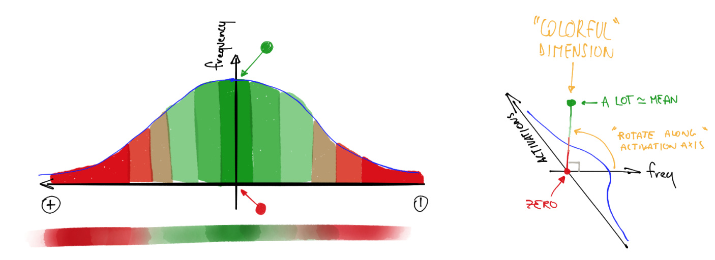
To create color_dim, we take the histogram shown on the left here, and convert it into just the colored representation shown at the bottom. Then we flip it on its side, as shown on the right. We found that the distribution is clearer if we take the log of the histogram values. Then, Stefano describes:
: The final plot for each layer is made by stacking the histogram of the activations from each batch along the horizontal axis. So each vertical slice in the visualisation represents the histogram of activations for a single batch. The color intensity corresponds to the height of the histogram, in other words the number of activations in each histogram bin.
<<colorful_summ>> shows how this all fits together.
为了创建color_dim,我们采用左侧显示的直方图,并将其转换为底部显示的彩色表示。然后我们将其翻转到右侧,如图所示。我们发现,如果我们对直方图值取对数,分布会更清晰。然后,Stefano描述:
:每个层的最终图是通过沿水平轴堆叠每个批量的激活直方图来制作的。因此可视化中的每个垂直切片代表单个批量的激活直方图。颜色强度对应直方图的高度,换句话说,就是每个直方图bin中的激活数量。
<<colorful_summ>>显示了这一切是如何结合在一起的。
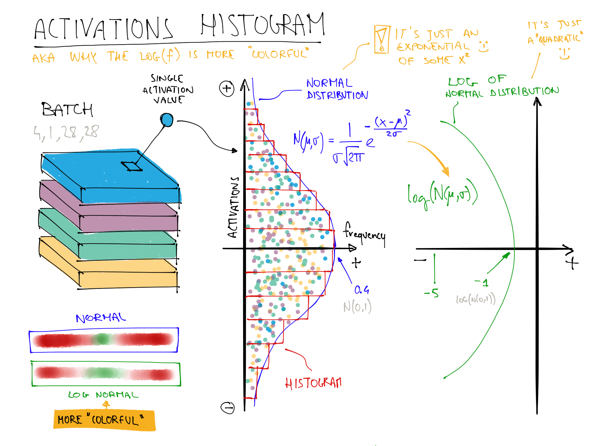
This illustrates why log(f) is more colorful than f when f follows a normal distribution because taking a log changes the Gaussian in a quadratic, which isn't as narrow.
这说明了为什么log(f)在f遵循正态分布时比f更丰富多彩,因为获取log会改变二次型中的高斯,而二次型没有那么窄。
So with that in mind, let's take another look at the result for the penultimate layer:
考虑到这一点,让我们再看看倒数第二层的结果:
learn.activation_stats.color_dim(-2)Output
<Figure size 720x360 with 1 Axes>
This shows a classic picture of "bad training." We start with nearly all activations at zero—that's what we see at the far left, with all the dark blue. The bright yellow at the bottom represents the near-zero activations. Then, over the first few batches we see the number of nonzero activations exponentially increasing. But it goes too far, and collapses! We see the dark blue return, and the bottom becomes bright yellow again. It almost looks like training restarts from scratch. Then we see the activations increase again, and collapse again. After repeating this a few times, eventually we see a spread of activations throughout the range.
It's much better if training can be smooth from the start. The cycles of exponential increase and then collapse tend to result in a lot of near-zero activations, resulting in slow training and poor final results. One way to solve this problem is to use batch normalization.
这是一张“糟糕的训练”的经典图片。我们从几乎所有的激活都是零开始——这就是我们在最左边看到的,所有的深蓝色。底部的亮黄色代表接近零的激活。然后,在前几批中,我们看到非零激活的数量呈指数级增长。但它走得太远了,然后崩溃了!我们看到深蓝色又回来了,底部又变成了亮黄色。这看起来就像是从头开始训练。然后我们看到激活再次增加,然后再次崩溃。重复几次后,最终我们看到整个范围的激活扩散。
如果训练一开始就能顺利进行就更好了。指数增长然后崩溃的循环往往会导致很多接近于零的激活,导致训练缓慢和最终结果糟糕。解决这个问题的一种方法是使用批标准化。
Batch Normalization
批标准化
To fix the slow training and poor final results we ended up with in the previous section, we need to fix the initial large percentage of near-zero activations, and then try to maintain a good distribution of activations throughout training.
Sergey Ioffe and Christian Szegedy presented a solution to this problem in the 2015 paper "Batch Normalization: Accelerating Deep Network Training by Reducing Internal Covariate Shift". In the abstract, they describe just the problem that we've seen:
: Training Deep Neural Networks is complicated by the fact that the distribution of each layer's inputs changes during training, as the parameters of the previous layers change. This slows down the training by requiring lower learning rates and careful parameter initialization... We refer to this phenomenon as internal covariate shift, and address the problem by normalizing layer inputs.
Their solution, they say is:
: Making normalization a part of the model architecture and performing the normalization for each training mini-batch. Batch Normalization allows us to use much higher learning rates and be less careful about initialization.
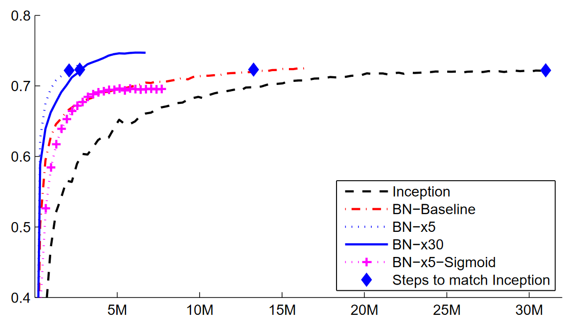
The paper caused great excitement as soon as it was released, because it included the chart in <>, which clearly demonstrated that batch normalization could train a model that was even more accurate than the current state of the art (the Inception architecture) and around 5x faster.
为了修复我们在上一节中结束的缓慢训练和糟糕的最终结果,我们需要修复初始的大百分比接近于零的激活,然后尝试在整个训练中保持良好的激活分布。
Sergey Ioffe和Christian Szegedy在2015年的论文“批标准化:通过减少内部协变量偏移来加速深度网络训练”中提出了这个问题的解决方案。抽象地说,他们描述的只是我们看到的问题:
:训练深度神经网络由于每个层的输入分布在训练期间随着前几层的参数变化而变化这一事实而变得复杂。这需要较低的学习率和仔细的参数初始化来减缓训练速度...我们将这种现象称为内部协变量移位,并通过标准化层输入来解决这个问题。
他们的解决方案是:
:将标准化作为模型体系结构的一部分,并对每个训练小批量执行标准化。批标准化允许我们使用更高的学习率,并且对初始化不那么小心。
这篇论文一发布就引起了极大的关注,因为它包含了<>中的图表,这清楚地证明了批标准化可以训练一个比当前最先进的模型(Inception架构)更准确且速度快5倍左右的模型。
Batch normalization (often just called batchnorm) works by taking an average of the mean and standard deviations of the activations of a layer and using those to normalize the activations. However, this can cause problems because the network might want some activations to be really high in order to make accurate predictions. So they also added two learnable parameters (meaning they will be updated in the SGD step), usually called gamma and beta. After normalizing the activations to get some new activation vector y, a batchnorm layer returns gamma*y + beta.
That's why our activations can have any mean or variance, independent from the mean and standard deviation of the results of the previous layer. Those statistics are learned separately, making training easier on our model. The behavior is different during training and validation: during training, we use the mean and standard deviation of the batch to normalize the data, while during validation we instead use a running mean of the statistics calculated during training.
Let's add a batchnorm layer to conv:
批标准化(通常称为batchnorm)的工作原理是取层激活的平均值和标准差的平均值,并使用它们来标准化激活。但是,这可能会导致问题,因为网络可能希望某些激活非常高,以便做出准确的预测。因此,他们还添加了两个可学习的参数(意味着它们将在SGD步骤中更新),通常称为gamma和beta。在标准化激活以获得一些新的激活向量y后,batchnorm层返回gamma*y + beta。
这就是为什么我们的激活可以有任何均值或方差,独立于前一层结果的均值和标准差。这些统计数据是单独学习的,使我们的模型更容易训练。在训练和验证期间,行为是不同的:在训练期间,我们使用批处理的均值和标准差来标准化数据,而在验证期间,我们使用训练期间计算的统计数据的运行平均值。
让我们在conv中添加一个batchnorm层:
def conv(ni, nf, ks=3, act=True):
    layers = [nn.Conv2d(ni, nf, stride=2, kernel_size=ks, padding=ks//2)]
    if act: layers.append(nn.ReLU())
    layers.append(nn.BatchNorm2d(nf))
    return nn.Sequential(*layers)
and fit our model:
符合我们的模型:
learn = fit()Output
<IPython.core.display.HTML object>
| epoch | train_loss | valid_loss | accuracy | time |
|---|---|---|---|---|
| 0 | 0.130036 | 0.055021 | 0.986400 | 00:10 |
That's a great result! Let's take a look at color_dim:
这是一个很好的结果!让我们看看color_dim:
learn.activation_stats.color_dim(-4)Output
<Figure size 720x360 with 1 Axes>

This is just what we hope to see: a smooth development of activations, with no "crashes." Batchnorm has really delivered on its promise here! In fact, batchnorm has been so successful that we see it (or something very similar) in nearly all modern neural networks.
An interesting observation about models containing batch normalization layers is that they tend to generalize better than models that don't contain them. Although we haven't as yet seen a rigorous analysis of what's going on here, most researchers believe that the reason for this is that batch normalization adds some extra randomness to the training process. Each mini-batch will have a somewhat different mean and standard deviation than other mini-batches. Therefore, the activations will be normalized by different values each time. In order for the model to make accurate predictions, it will have to learn to become robust to these variations. In general, adding additional randomization to the training process often helps.
Since things are going so well, let's train for a few more epochs and see how it goes. In fact, let's increase the learning rate, since the abstract of the batchnorm paper claimed we should be able to "train at much higher learning rates":
这正是我们希望看到的:激活的平稳发展,没有“崩溃”。BatchNorm在这里真的兑现了它的承诺!事实上,batchNorm非常成功,以至于我们在几乎所有现代神经网络中都看到了它(或类似的东西)。
关于包含批标准化层的模型,一个有趣的观察是,它们往往比不包含它们的模型更容易泛化。虽然我们还没有看到对这里发生了什么进行严格的分析,但大多数研究人员认为,这是因为批标准化为训练过程增加了一些额外的随机性。每个小批量都会比其他小批量有一些不同的均值和标准差。因此,每次激活都会被不同的值标准化。为了让模型做出准确的预测,它必须学会对这些变化变得健壮。一般来说,在训练过程中加入额外的随机性通常会有所帮助。
既然事情进展得如此顺利,让我们再训练几轮,看看进展如何。事实上,让我们提高学习率,因为batchnorm论文的摘要声称我们应该能够“以更高的学习率进行训练”:
learn = fit(5, lr=0.1)Output
<IPython.core.display.HTML object>
| epoch | train_loss | valid_loss | accuracy | time |
|---|---|---|---|---|
| 0 | 0.191731 | 0.121738 | 0.960900 | 00:11 |
| 1 | 0.083739 | 0.055808 | 0.981800 | 00:10 |
| 2 | 0.053161 | 0.044485 | 0.987100 | 00:10 |
| 3 | 0.034433 | 0.030233 | 0.990200 | 00:10 |
| 4 | 0.017646 | 0.025407 | 0.991200 | 00:10 |
At this point, I think it's fair to say we know how to recognize digits! It's time to move on to something harder...
在这一点上,我认为可以公平地说我们知道如何识别数字!是时候转向更难的东西了......
Conclusions
结论
We've seen that convolutions are just a type of matrix multiplication, with two constraints on the weight matrix: some elements are always zero, and some elements are tied (forced to always have the same value). In <<chapter_intro>> we saw the eight requirements from the 1986 book Parallel Distributed Processing; one of them was "A pattern of connectivity among units." That's exactly what these constraints do: they enforce a certain pattern of connectivity.
These constraints allow us to use far fewer parameters in our model, without sacrificing the ability to represent complex visual features. That means we can train deeper models faster, with less overfitting. Although the universal approximation theorem shows that it should be possible to represent anything in a fully connected network in one hidden layer, we've seen now that in practice we can train much better models by being thoughtful about network architecture.
Convolutions are by far the most common pattern of connectivity we see in neural nets (along with regular linear layers, which we refer to as fully connected), but it's likely that many more will be discovered.
We've also seen how to interpret the activations of layers in the network to see whether training is going well or not, and how batchnorm helps regularize the training and makes it smoother. In the next chapter, we will use both of those layers to build the most popular architecture in computer vision: a residual network.
我们已经看到卷积只是一种矩阵乘法,对权重矩阵有两个约束:一些元素始终为零,一些元素是并列的(被迫始终具有相同的值)。在<<chapter_intro>>中,我们看到了1986年《并行分布式处理》一书中的八个要求;其中一个是“单元之间的连接模式”。这正是这些约束的作用:它们强制执行某种连接模式。
这些约束允许我们在模型中使用更少的参数,而不会牺牲表示复杂视觉特征的能力。这意味着我们可以更快地训练更深层次的模型,而不会过度拟合。尽管通用近似定理表明,在一个隐藏层中表示完全连接的网络中的任何东西都应该是可能的,但我们现在已经看到,在实践中,我们可以通过仔细考虑网络架构来训练更好的模型。
到目前为止,卷积是我们在神经网络中看到的最常见的连接模式(以及常规的线性层,我们称之为完全连接),但很可能会发现更多的连接模式。
我们还了解了如何解释网络层的激活,以查看训练是否进行得很顺利,以及batchnorm如何帮助正则化训练并使其更流畅。在下一章中,我们将使用这两个层来构建计算机视觉中最流行的架构:残差网络。
Questionnaire
问卷
- What is a "feature"?
- Write out the convolutional kernel matrix for a top edge detector.
- Write out the mathematical operation applied by a 3×3 kernel to a single pixel in an image.
- What is the value of a convolutional kernel apply to a 3×3 matrix of zeros?
- What is "padding"?
- What is "stride"?
- Create a nested list comprehension to complete any task that you choose.
- What are the shapes of the
inputandweightparameters to PyTorch's 2D convolution? - What is a "channel"?
- What is the relationship between a convolution and a matrix multiplication?
- What is a "convolutional neural network"?
- What is the benefit of refactoring parts of your neural network definition?
- What is
Flatten? Where does it need to be included in the MNIST CNN? Why? - What does "NCHW" mean?
- Why does the third layer of the MNIST CNN have
7*7*(1168-16)multiplications? - What is a "receptive field"?
- What is the size of the receptive field of an activation after two stride 2 convolutions? Why?
- Run conv-example.xlsx yourself and experiment with trace precedents.
- Have a look at Jeremy or Sylvain's list of recent Twitter "like"s, and see if you find any interesting resources or ideas there.
- How is a color image represented as a tensor?
- How does a convolution work with a color input?
- What method can we use to see that data in
DataLoaders? - Why do we double the number of filters after each stride-2 conv?
- Why do we use a larger kernel in the first conv with MNIST (with
simple_cnn)? - What information does
ActivationStatssave for each layer? - How can we access a learner's callback after training?
- What are the three statistics plotted by
plot_layer_stats? What does the x-axis represent? - Why are activations near zero problematic?
- What are the upsides and downsides of training with a larger batch size?
- Why should we avoid using a high learning rate at the start of training?
- What is 1cycle training?
- What are the benefits of training with a high learning rate?
- Why do we want to use a low learning rate at the end of training?
- What is "cyclical momentum"?
- What callback tracks hyperparameter values during training (along with other information)?
- What does one column of pixels in the
color_dimplot represent? - What does "bad training" look like in
color_dim? Why? - What trainable parameters does a batch normalization layer contain?
- What statistics are used to normalize in batch normalization during training? How about during validation?
- Why do models with batch normalization layers generalize better?
- 什么是“特征”?
- 写出一个上边缘检测器的卷积核矩阵。
- 写出3×3卷积核应用于图像中单个像素的数学运算。
- 卷积核应用于3×3零矩阵的值是多少?
- 什么是“填充”?
- 什么是“步幅”?
- 创建嵌套列表推导式来完成您选择的任何任务。
- PyTorch的2D卷积的
input和weight参数的形状是什么? - 什么是“通道”?
- 卷积和矩阵乘法有什么关系?
- 什么是“卷积神经网络”?
- 重构你的神经网络定义的部分有什么好处?
- 什么是
Flatten?它需要包含在MNIST CNN的哪里?为什么? - “NCHW”是什么意思?
- 为什么MNIST CNN的第三层有
7*7*(1168-16)乘法? - 什么是“感受野”?
- 在两个stride-2卷积后,激活的感受野的大小是多少?为什么?
- 自己运行conv-example.xlsx并尝试跟踪先例。
- 看看Jeremy或Sylvain最近的推特“喜欢”列表,看看你是否在那里找到任何有趣的资源或想法。
- 彩色图像如何表示为张量?
- 卷积如何与颜色输入一起工作?
- 我们可以使用什么方法在
DataLoaders中查看该数据? - 为什么我们在每次stride-2卷积后要将过滤器的数量增加一倍?
- 为什么我们在MNIST的第一个卷积中使用更大的卷积核(带有
simple_cnn)? - “ActivationStats”为每一层保存哪些信息?
- 我们如何在训练后访问learner的回调?
plot_layer_stats绘制的三个统计数据是什么?x轴代表什么?- 为什么接近零的激活会有问题?
- 批量更大的训练有什么好处和坏处?
- 为什么我们要避免在训练开始时使用高学习率?
- 什么是1周期训练?
- 学习率高的训练有什么好处?
- 为什么我们要在训练结束时使用低学习率?
- 什么是“周期动量”?
- 哪些回调在训练期间跟踪超参数值(以及其他信息)?
color_dim图中的一列像素代表什么?- “糟糕的训练”在
color_dim中是什么样子的?为什么? - 批标准化层包含哪些可训练参数?
- 训练时批标准化中使用哪些统计数据进行标准化?在验证期间呢?
- 为什么批标准化层的模型泛化得更好?
Further Research
进一步研究
- What features other than edge detectors have been used in computer vision (especially before deep learning became popular)?
- There are other normalization layers available in PyTorch. Try them out and see what works best. Learn about why other normalization layers have been developed, and how they differ from batch normalization.
- Try moving the activation function after the batch normalization layer in
conv. Does it make a difference? See what you can find out about what order is recommended, and why.
- 除了边缘检测器之外,计算机视觉还使用了哪些特征(尤其是在深度学习流行之前)?
- PyTorch中还有其他可用的规范化层。尝试一下,看看什么最有效。了解为什么开发了其他规范化层,以及它们与批处理规范化有何不同。
- 尝试在
conv中的批处理规范化层之后移动激活函数。有区别吗?看看你能找到什么关于推荐顺序的信息,以及为什么。