
Chapter 15
Application Architectures Deep Dive
#hide
! [ -e /content ] && pip install -Uqq fastbook
import fastbook
fastbook.setup_book()#hide
from fastbook import *Application Architectures Deep Dive
应用架构深入探讨
We are now in the exciting position that we can fully understand the architectures that we have been using for our state-of-the-art models for computer vision, natural language processing, and tabular analysis. In this chapter, we're going to fill in all the missing details on how fastai's application models work and show you how to build the models they use.
We will also go back to the custom data preprocessing pipeline we saw in <<chapter_midlevel_data>> for Siamese networks and show you how you can use the components in the fastai library to build custom pretrained models for new tasks.
We'll start with computer vision.
我们现在处于令人兴奋的位置,我们可以完全理解我们一直在用于计算机视觉、自然语言处理和表格分析的最先进模型的架构。在本章中,我们将填补有关 fastai 应用程序模型如何工作的所有缺失细节,并向您展示如何构建它们使用的模型。
我们还将回到我们在 《chapter_midlevel_data》 中看到的用于连体网络的自定义数据预处理管道,并向您展示如何使用 fastai 库中的组件为新任务构建自定义预训练模型。
我们将从计算机视觉开始。
Computer Vision
计算机视觉
For computer vision application we use the functions vision_learner and unet_learner to build our models, depending on the task. In this section we'll explore how to build the Learner objects we used in Parts 1 and 2 of this book.
对于计算机视觉应用,我们使用函数 vision_learner 和 unet_learner 来构建我们的模型,具体取决于任务。在本节中,我们将探讨如何构建我们在本书第 1 部分和第 2 部分中使用的 Learner 对象。
vision_learner
视觉学习者
Let's take a look at what happens when we use the vision_learner function. We begin by passing this function an architecture to use for the body of the network. Most of the time we use a ResNet, which you already know how to create, so we don't need to delve into that any further. Pretrained weights are downloaded as required and loaded into the ResNet.
Then, for transfer learning, the network needs to be cut. This refers to slicing off the final layer, which is only responsible for ImageNet-specific categorization. In fact, we do not slice off only this layer, but everything from the adaptive average pooling layer onwards. The reason for this will become clear in just a moment. Since different architectures might use different types of pooling layers, or even completely different kinds of heads, we don't just search for the adaptive pooling layer to decide where to cut the pretrained model. Instead, we have a dictionary of information that is used for each model to determine where its body ends, and its head starts. We call this model_meta—here it is for resnet-50:
让我们看看当我们使用 vision_learner 函数时会发生什么。我们首先将这个函数传递给用于网络主体的架构。大多数时候我们使用 ResNet,你已经知道如何创建它,所以我们不需要进一步深入研究。根据需要下载预训练的权重并加载到 ResNet。
然后,对于迁移学习,需要切断网络。这是指切掉最后一层,它只负责 ImageNet 特定的分类。事实上,我们不只是切掉这一层,而是从自适应平均池化层开始的所有内容。其原因将在一瞬间变得清晰。由于不同的架构可能使用不同类型的池化层,甚至完全不同的头,我们不只是搜索自适应池化层来决定在哪里切割预训练模型。相反,我们有一个信息字典,用于每个模型来确定它的身体在哪里结束,它的头部从哪里开始。我们称之为 model_meta ——这里是 resnet-50:
model_meta[resnet50]Output
{'cut': -2,
 'split': <function fastai.vision.learner._resnet_split(m)>,
 'stats': ([0.485, 0.456, 0.406], [0.229, 0.224, 0.225])}
jargon: Body and Head: The "head" of a neural net is the part that is specialized for a particular task. For a CNN, it's generally the part after the adaptive average pooling layer. The "body" is everything else, and includes the "stem" (which we learned about in <<chapter_resnet>>).
行话:身体和头部:神经网络的“头部”是专门用于特定任务的部分。对于 CNN,它通常是自适应平均池化层之后的部分。 “body”就是其他一切,包括“stem”(我们在 《chapter_resnet》 中了解到)。
If we take all of the layers prior to the cut point of -2, we get the part of the model that fastai will keep for transfer learning. Now, we put on our new head. This is created using the function create_head:
如果我们在 -2 的切点之前获取所有层,我们将得到 fastai 将保留用于迁移学习的模型部分。现在,我们换上了新的头。这是使用函数 create_head 创建的:
#hide_output
create_head(20,2)
Output
Sequential(
  (0): AdaptiveConcatPool2d(
    (ap): AdaptiveAvgPool2d(output_size=1)
    (mp): AdaptiveMaxPool2d(output_size=1)
  )
  (1): full: False
  (2): BatchNorm1d(20, eps=1e-05, momentum=0.1, affine=True, track_running_stats=True)
  (3): Dropout(p=0.25, inplace=False)
  (4): Linear(in_features=20, out_features=512, bias=False)
  (5): ReLU(inplace=True)
  (6): BatchNorm1d(512, eps=1e-05, momentum=0.1, affine=True, track_running_stats=True)
  (7): Dropout(p=0.5, inplace=False)
  (8): Linear(in_features=512, out_features=2, bias=False)
)Sequential(
(0): AdaptiveConcatPool2d(
(ap): AdaptiveAvgPool2d(output_size=1)
(mp): AdaptiveMaxPool2d(output_size=1)
)
(1): Flatten()
(2): BatchNorm1d(20, eps=1e-05, momentum=0.1, affine=True)
(3): Dropout(p=0.25, inplace=False)
(4): Linear(in_features=20, out_features=512, bias=False)
(5): ReLU(inplace=True)
(6): BatchNorm1d(512, eps=1e-05, momentum=0.1, affine=True)
(7): Dropout(p=0.5, inplace=False)
(8): Linear(in_features=512, out_features=2, bias=False)
)With this function you can choose how many additional linear layers are added to the end, how much dropout to use after each one, and what kind of pooling to use. By default, fastai will apply both average pooling, and max pooling, and will concatenate the two together (this is the AdaptiveConcatPool2d layer). This is not a particularly common approach, but it was developed independently at fastai and other research labs in recent years, and tends to provide some small improvement over using just average pooling.
fastai is a bit different from most libraries in that by default it adds two linear layers, rather than one, in the CNN head. The reason for this is that transfer learning can still be useful even, as we have seen, when transferring the pretrained model to very different domains. However, just using a single linear layer is unlikely to be enough in these cases; we have found that using two linear layers can allow transfer learning to be used more quickly and easily, in more situations.
使用此功能,您可以选择在最后添加多少额外的线性层,在每个层之后使用多少 dropout,以及使用哪种池化。默认情况下,fastai 将同时应用平均池化和最大池化,并将两者连接在一起(这是 AdaptiveConcatPool2d 层)。这不是一种特别常见的方法,但它是近年来在 fastai 和其他研究实验室独立开发的,并且往往比仅使用平均池化提供一些小的改进。
fastai 与大多数库有点不同,默认情况下它在 CNN 头部添加了两个线性层,而不是一个。这样做的原因是,即使如我们所见,将预训练模型转移到非常不同的领域时,转移学习仍然有用。但是,在这些情况下,仅使用单个线性层是不够的;我们发现,使用两个线性层可以在更多情况下更快速、更轻松地使用迁移学习。
note: One Last Batchnorm?: One parameter to
create_headthat is worth looking at isbn_final. Setting this totruewill cause a batchnorm layer to be added as your final layer. This can be useful in helping your model scale appropriately for your output activations. We haven't seen this approach published anywhere as yet, but we have found that it works well in practice wherever we have used it.
注意:One Last Batchnorm?:create_head 的一个值得关注的参数是 bn_final。将此设置为 true 将导致添加一个 batchnorm 层作为您的最终层。这有助于帮助您的模型针对输出激活进行适当缩放。我们还没有看到这种方法在任何地方发布,但是我们发现它在我们使用它的任何地方都可以很好地工作。
Let's now take a look at what unet_learner did in the segmentation problem we showed in <<chapter_intro>>.
现在让我们看看 unet_learner 在 《chapter_intro》 中展示的分割问题中做了什么。
unet_learner
unet 学者
One of the most interesting architectures in deep learning is the one that we used for segmentation in <<chapter_intro>>. Segmentation is a challenging task, because the output required is really an image, or a pixel grid, containing the predicted label for every pixel. There are other tasks that share a similar basic design, such as increasing the resolution of an image (super-resolution), adding color to a black-and-white image (colorization), or converting a photo into a synthetic painting (style transfer)—these tasks are covered by an online chapter of this book, so be sure to check it out after you've read this chapter. In each case, we are starting with an image and converting it to some other image of the same dimensions or aspect ratio, but with the pixels altered in some way. We refer to these as generative vision models.
The way we do this is to start with the exact same approach to developing a CNN head as we saw in the previous problem. We start with a ResNet, for instance, and cut off the adaptive pooling layer and everything after that. Then we replace those layers with our custom head, which does the generative task.
There was a lot of handwaving in that last sentence! How on earth do we create a CNN head that generates an image? If we start with, say, a 224-pixel input image, then at the end of the ResNet body we will have a 7×7 grid of convolutional activations. How can we convert that into a 224-pixel segmentation mask?
Naturally, we do this with a neural network! So we need some kind of layer that can increase the grid size in a CNN. One very simple approach to this is to replace every pixel in the 7×7 grid with four pixels in a 2×2 square. Each of those four pixels will have the same value—this is known as nearest neighbor interpolation. PyTorch provides a layer that does this for us, so one option is to create a head that contains stride-1 convolutional layers (along with batchnorm and ReLU layers as usual) interspersed with 2×2 nearest neighbor interpolation layers. In fact, you can try this now! See if you can create a custom head designed like this, and try it on the CamVid segmentation task. You should find that you get some reasonable results, although they won't be as good as our <<chapter_intro>> results.
Another approach is to replace the nearest neighbor and convolution combination with a transposed convolution, otherwise known as a stride half convolution. This is identical to a regular convolution, but first zero padding is inserted between all the pixels in the input. This is easiest to see with a picture—<<transp_conv>> shows a diagram from the excellent convolutional arithmetic paper we discussed in <<chapter_convolutions>>, showing a 3×3 transposed convolution applied to a 3×3 image.
深度学习中最有趣的架构之一是我们在 《chapter_intro》 中用于分割的架构。分割是一项具有挑战性的任务,因为所需的输出实际上是图像或像素网格,其中包含每个像素的预测标签。还有其他任务共享类似的基本设计,例如提高图像的分辨率(超分辨率),为黑白图像添加颜色(着色),或将照片转换为合成绘画(风格转换)——本书的在线章节涵盖了这些任务,因此请务必在阅读完本章后查看。在每种情况下,我们都从一个图像开始,并将其转换为具有相同尺寸或纵横比的其他图像,但像素以某种方式改变。我们将这些称为生成视觉模型。
我们这样做的方法是从与我们在上一个问题中看到的完全相同的方法开始开发 CNN 头部。例如,我们从 ResNet 开始,然后切断自适应池化层和之后的所有内容。然后我们用我们的自定义头替换这些层,它执行生成任务。
最后一句话里有很多挥手的意思!我们到底如何创建一个生成图像的 CNN 头部?如果我们从一个 224 像素的输入图像开始,那么在 ResNet 主体的末尾,我们将有一个 7×7 的卷积激活网格。我们如何将其转换为 224 像素的分割蒙版?
当然,我们使用神经网络来做到这一点!所以我们需要某种层来增加 CNN 中的网格大小。一种非常简单的方法是将 7×7 网格中的每个像素替换为 2×2 正方形中的四个像素。这四个像素中的每一个都将具有相同的值——这称为最近邻插值。 PyTorch 为我们提供了一个层,因此一个选择是创建一个包含 stride-1 卷积层(以及通常的 batchnorm 和 ReLU 层)的头部,其中散布有 2×2 最近邻插值层。事实上,你现在可以试试这个!看看你是否可以创建一个这样设计的自定义头部,并在 CamVid 分割任务上进行尝试。你应该会发现你得到了一些合理的结果,尽管它们不会像我们的 《chapter_intro》 结果那么好。
另一种方法是用转置卷积代替最近邻和卷积组合,也称为跨步半卷积。这与常规卷积相同,但首先在输入中的所有像素之间插入零填充。用图片最容易看出这一点——《transp_conv》 显示了我们在 《chapter_convolutions》 中讨论的优秀卷积算术论文中的图表,显示了应用于 3×3 图像的 3×3 转置卷积。
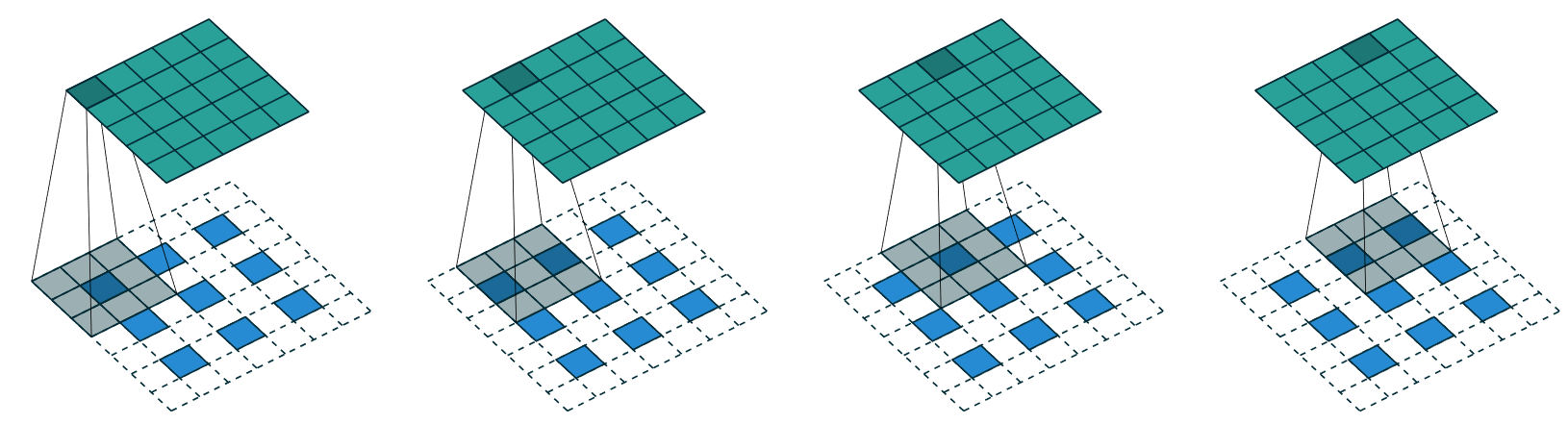
As you see, the result of this is to increase the size of the input. You can try this out now by using fastai's ConvLayer class; pass the parameter transpose=True to create a transposed convolution, instead of a regular one, in your custom head.
Neither of these approaches, however, works really well. The problem is that our 7×7 grid simply doesn't have enough information to create a 224×224-pixel output. It's asking an awful lot of the activations of each of those grid cells to have enough information to fully regenerate every pixel in the output. The solution to this problem is to use skip connections, like in a ResNet, but skipping from the activations in the body of the ResNet all the way over to the activations of the transposed convolution on the opposite side of the architecture. This approach, illustrated in <>, was developed by Olaf Ronneberger, Philipp Fischer, and Thomas Brox in the 2015 paper "U-Net: Convolutional Networks for Biomedical Image Segmentation". Although the paper focused on medical applications, the U-Net has revolutionized all kinds of generative vision models.
如您所见,这样做的结果是增加了输入的大小。您现在可以使用 fastai 的 ConvLayer 类来尝试一下;传递参数 transpose=True 以在您的自定义头部中创建转置卷积,而不是常规卷积。
然而,这两种方法都不是很好。问题是我们的 7×7 网格根本没有足够的信息来创建 224×224 像素的输出。它要求每个网格单元的大量激活具有足够的信息来完全重新生成输出中的每个像素。这个问题的解决方案是使用跳跃连接,就像在 ResNet 中一样,但是从 ResNet 主体中的激活一直跳过到架构另一侧的转置卷积的激活。 《unet》 中说明的这种方法是由 Olaf Ronneberger、Philipp Fischer 和 Thomas Brox 在 2015 年的论文“U-Net: Convolutional Networks for Biomedical Image Segmentation”中开发的。尽管这篇论文专注于医疗应用,但 U-Net 已经彻底改变了各种生成视觉模型。
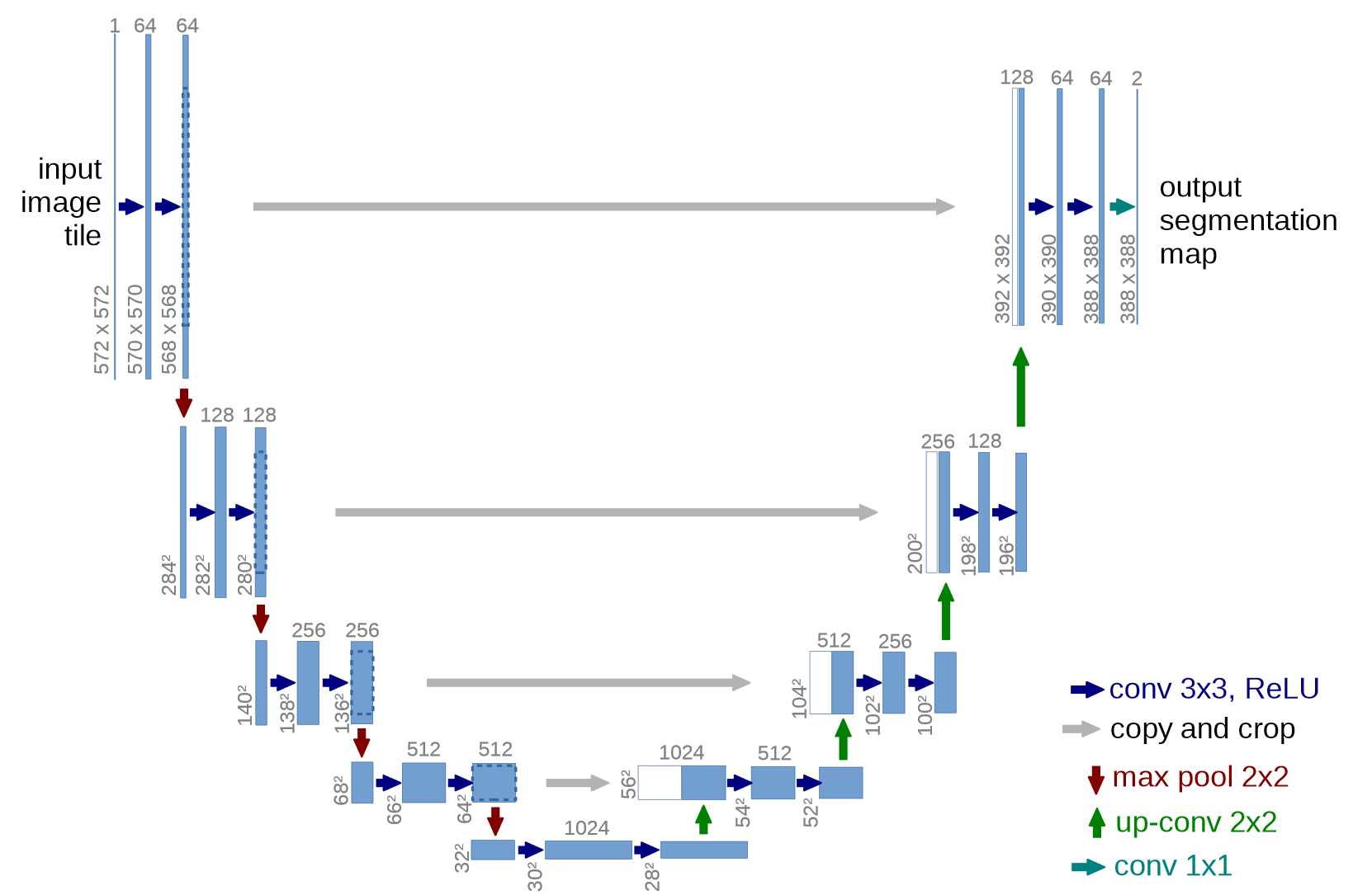
This picture shows the CNN body on the left (in this case, it's a regular CNN, not a ResNet, and they're using 2×2 max pooling instead of stride-2 convolutions, since this paper was written before ResNets came along) and the transposed convolutional ("up-conv") layers on the right. Then extra skip connections are shown as gray arrows crossing from left to right (these are sometimes called cross connections). You can see why it's called a "U-Net!"
With this architecture, the input to the transposed convolutions is not just the lower-resolution grid in the preceding layer, but also the higher-resolution grid in the ResNet head. This allows the U-Net to use all of the information of the original image, as it is needed. One challenge with U-Nets is that the exact architecture depends on the image size. fastai has a unique DynamicUnet class that autogenerates an architecture of the right size based on the data provided.
Let's focus now on an example where we leverage the fastai library to write a custom model.
这张图片显示了左侧的 CNN 主体(在这种情况下,它是一个常规的 CNN,而不是 ResNet,并且他们使用 2×2 最大池而不是 stride-2 卷积,因为这篇论文是在 ResNet 出现之前写的)以及右侧的转置卷积(“up-conv”)层。然后额外的跳过连接显示为从左到右交叉的灰色箭头(这些有时称为交叉连接)。您可以看到为什么它被称为“U-Net!”
使用这种架构,转置卷积的输入不仅是前一层中较低分辨率的网格,还有 ResNet 头部中的较高分辨率网格。这允许 U-Net 根据需要使用原始图像的所有信息。 U-Nets 的一个挑战是确切的架构取决于图像大小。 fastai 有一个独特的 DynamicUnet 类,可以根据提供的数据自动生成合适大小的架构。
现在让我们关注一个利用 fastai 库编写自定义模型的示例。
A Siamese Network
#hide
from fastai.vision.all import *
path = untar_data(URLs.PETS)
files = get_image_files(path/"images")

class SiameseImage(fastuple):
    def show(self, ctx=None, **kwargs):
        img1,img2,same_breed = self
        if not isinstance(img1, Tensor):
            if img2.size != img1.size: img2 = img2.resize(img1.size)
            t1,t2 = tensor(img1),tensor(img2)
            t1,t2 = t1.permute(2,0,1),t2.permute(2,0,1)
        else: t1,t2 = img1,img2
        line = t1.new_zeros(t1.shape[0], t1.shape[1], 10)
        return show_image(torch.cat([t1,line,t2], dim=2),
                          title=same_breed, ctx=ctx)

def label_func(fname):
    return re.match(r'^(.*)_\d+.jpg$', fname.name).groups()[0]

class SiameseTransform(Transform):
    def __init__(self, files, label_func, splits):
        self.labels = files.map(label_func).unique()
        self.lbl2files = {l: L(f for f in files if label_func(f) == l) for l in self.labels}
        self.label_func = label_func
        self.valid = {f: self._draw(f) for f in files[splits[1]]}

    def encodes(self, f):
        f2,t = self.valid.get(f, self._draw(f))
        img1,img2 = PILImage.create(f),PILImage.create(f2)
        return SiameseImage(img1, img2, t)

    def _draw(self, f):
        same = random.random() < 0.5
        cls = self.label_func(f)
        if not same: cls = random.choice(L(l for l in self.labels if l != cls))
        return random.choice(self.lbl2files[cls]),same

splits = RandomSplitter()(files)
tfm = SiameseTransform(files, label_func, splits)
tls = TfmdLists(files, tfm, splits=splits)
dls = tls.dataloaders(after_item=[Resize(224), ToTensor],
    after_batch=[IntToFloatTensor, Normalize.from_stats(*imagenet_stats)])
Let's go back to the input pipeline we set up in <<chapter_midlevel_data>> for a Siamese network. If you remember, it consisted of pair of images with the label being True or False, depending on if they were in the same class or not.
Using what we just saw, let's build a custom model for this task and train it. How? We will use a pretrained architecture and pass our two images through it. Then we can concatenate the results and send them to a custom head that will return two predictions. In terms of modules, this looks like this:
让我们回到我们在 <> 中为连体网络设置的输入管道。如果您还记得,它由标签为 True 或 False 的一对图像组成,具体取决于它们是否属于同一类。
使用我们刚刚看到的内容,让我们为此任务构建一个自定义模型并对其进行训练。如何?我们将使用预训练的架构并通过它传递我们的两个图像。然后我们可以连接结果并将它们发送到一个自定义头部,该头部将返回两个预测。在模块方面,这看起来像这样:
class SiameseModel(Module):
    def __init__(self, encoder, head):
        self.encoder,self.head = encoder,head

    def forward(self, x1, x2):
        ftrs = torch.cat([self.encoder(x1), self.encoder(x2)], dim=1)
        return self.head(ftrs)
To create our encoder, we just need to take a pretrained model and cut it, as we explained before. The function create_body does that for us; we just have to pass it the place where we want to cut. As we saw earlier, per the dictionary of metadata for pretrained models, the cut value for a resnet is -2:
如前所述,要创建我们的编码器,我们只需要采用预训练模型并对其进行剪切即可。函数 create_body 为我们做这件事;我们只需要将它传递到我们想要剪切的地方。正如我们之前看到的,根据预训练模型的元数据字典,resnet 的切割值为 -2:
encoder = create_body(resnet34, cut=-2)Then we can create our head. A look at the encoder tells us the last layer has 512 features, so this head will need to receive 512*2. Why 2? We have to multiply by 2 because we have two images. So we create the head as follows:
然后我们可以创建我们的头。看一下编码器告诉我们最后一层有 512 个特征,所以这个头需要接收 512*2。为什么是2?我们必须乘以 2,因为我们有两个图像。所以我们创建头部如下:
head = create_head(512*2, 2, ps=0.5)With our encoder and head, we can now build our model:
使用我们的编码器和头部,我们现在可以构建我们的模型:
model = SiameseModel(encoder, head)Before using Learner, we have two more things to define. First, we must define the loss function we want to use. It's regular cross-entropy, but since our targets are Booleans, we need to convert them to integers or PyTorch will throw an error:
Before using Learner, we have two more things to define. First, we must define the loss function we want to use. It's regular cross-entropy, but since our targets are Booleans, we need to convert them to integers or PyTorch will throw an error:
def loss_func(out, targ):
    return nn.CrossEntropyLoss()(out, targ.long())
More importantly, to take full advantage of transfer learning, we have to define a custom splitter. A splitter is a function that tells the fastai library how to split the model into parameter groups. These are used behind the scenes to train only the head of a model when we do transfer learning.
Here we want two parameter groups: one for the encoder and one for the head. We can thus define the following splitter (params is just a function that returns all parameters of a given module):
更重要的是,要充分利用迁移学习,我们必须定义一个自定义拆分器。拆分器是一个函数,它告诉 fastai 库如何将模型拆分为参数组。当我们进行迁移学习时,这些在幕后仅用于训练模型的头部。
这里我们需要两个参数组:一个用于编码器,一个用于磁头。因此,我们可以定义以下拆分器(params 只是一个返回给定模块的所有参数的函数):
def siamese_splitter(model):
    return [params(model.encoder), params(model.head)]
Then we can define our Learner by passing the data, model, loss function, splitter, and any metric we want. Since we are not using a convenience function from fastai for transfer learning (like vision_learner), we have to call learn.freeze manually. This will make sure only the last parameter group (in this case, the head) is trained:
然后我们可以通过传递数据、模型、损失函数、拆分器和任何我们想要的指标来定义我们的learner。由于我们没有使用 fastai 的便捷函数进行迁移学习(如 vision_learner),我们必须手动调用 learn.freeze。这将确保只训练最后一个参数组(在本例中为头部):
learn = Learner(dls, model, loss_func=loss_func,
                splitter=siamese_splitter, metrics=accuracy)
learn.freeze()
Then we can directly train our model with the usual methods:
然后我们可以直接用常用的方法训练我们的模型:
learn.fit_one_cycle(4, 3e-3)Output
<IPython.core.display.HTML object>
| epoch | train_loss | valid_loss | accuracy | time |
|---|---|---|---|---|
| 0 | 0.367015 | 0.281242 | 0.885656 | 00:26 |
| 1 | 0.307688 | 0.214721 | 0.915426 | 00:26 |
| 2 | 0.275221 | 0.170615 | 0.936401 | 00:26 |
| 3 | 0.223771 | 0.159633 | 0.943843 | 00:26 |
Before unfreezing and fine-tuning the whole model a bit more with discriminative learning rates (that is: a lower learning rate for the body and a higher one for the head):
在解冻和微调整个模型之前,使用判别学习率(即:身体的学习率较低,头部的学习率较高):
learn.unfreeze()
learn.fit_one_cycle(4, slice(1e-6,1e-4))
Output
<IPython.core.display.HTML object>
| epoch | train_loss | valid_loss | accuracy | time |
|---|---|---|---|---|
| 0 | 0.212744 | 0.159033 | 0.944520 | 00:35 |
| 1 | 0.201893 | 0.159615 | 0.942490 | 00:35 |
| 2 | 0.204606 | 0.152338 | 0.945196 | 00:36 |
| 3 | 0.213203 | 0.148346 | 0.947903 | 00:36 |
94.8% is very good when we remember a classifier trained the same way (with no data augmentation) had an error rate of 7%.
当我们记得以相同方式训练的分类器(没有数据增强)有 7% 的错误率时,94.8% 非常好。
Now that we've seen how to create complete state-of-the-art computer vision models, let's move on to NLP.
现在我们已经了解了如何创建完整的最先进的计算机视觉模型,让我们继续讨论 NLP。
Natural Language Processing
自然语言处理
Converting an AWD-LSTM language model into a transfer learning classifier, as we did in <<chapter_nlp>>, follows a very similar process to what we did with vision_learner in the first section of this chapter. We do not need a "meta" dictionary in this case, because we do not have such a variety of architectures to support in the body. All we need to do is select the stacked RNN for the encoder in the language model, which is a single PyTorch module. This encoder will provide an activation for every word of the input, because a language model needs to output a prediction for every next word.
To create a classifier from this we use an approach described in the ULMFiT paper as "BPTT for Text Classification (BPT3C)":
将 AWD-LSTM 语言模型转换为迁移学习分类器,就像我们在 《chapter_nlp》 中所做的那样,遵循与本章第一节中使用 vision_learner 所做的非常相似的过程。在这种情况下,我们不需要“元”字典,因为我们体内没有这么多种架构可以支持。我们需要做的就是在语言模型中为编码器选择堆叠的 RNN,这是一个单一的 PyTorch 模块。该编码器将为输入的每个单词提供激活,因为语言模型需要为每个下一个单词输出预测。
为了创建一个分类器,我们使用 ULMFiT 论文中描述的方法“BPTT for Text Classification (BPT3C)”:
: We divide the document into fixed-length batches of size b. At the beginning of each batch, the model is initialized with the final state of the previous batch; we keep track of the hidden states for mean and max-pooling; gradients are back-propagated to the batches whose hidden states contributed to the final prediction. In practice, we use variable length backpropagation sequences.
:我们将文档分成大小为 b 的固定长度的批次。在每批开始时,使用前一批的最终状态初始化模型;我们跟踪平均池和最大池的隐藏状态;梯度被反向传播到隐藏状态对最终预测有贡献的批次。在实践中,我们使用可变长度反向传播序列。
In other words, the classifier contains a for loop, which loops over each batch of a sequence. The state is maintained across batches, and the activations of each batch are stored. At the end, we use the same average and max concatenated pooling trick that we use for computer vision models—but this time, we do not pool over CNN grid cells, but over RNN sequences.
For this for loop we need to gather our data in batches, but each text needs to be treated separately, as they each have their own labels. However, it's very likely that those texts won't all be of the same length, which means we won't be able to put them all in the same array, like we did with the language model.
That's where padding is going to help: when grabbing a bunch of texts, we determine the one with the greatest length, then we fill the ones that are shorter with a special token called xxpad. To avoid extreme cases where we have a text with 2,000 tokens in the same batch as a text with 10 tokens (so a lot of padding, and a lot of wasted computation), we alter the randomness by making sure texts of comparable size are put together. The texts will still be in a somewhat random order for the training set (for the validation set we can simply sort them by order of length), but not completely so.
This is done automatically behind the scenes by the fastai library when creating our DataLoaders.
换句话说,分类器包含一个 for 循环,该循环遍历序列的每批。跨批次维护状态,并存储每个批次的激活。最后,我们使用与计算机视觉模型相同的平均和最大级联池化技巧——但这一次,我们不是在 CNN 网格单元上池化,而是在 RNN 序列上池化。
对于这个 for 循环,我们需要分批收集数据,但是每个文本都需要单独处理,因为它们都有自己的标签。但是,很可能这些文本的长度不同,这意味着我们无法将它们全部放在同一个数组中,就像我们对语言模型所做的那样。
这就是填充的作用:当抓取一堆文本时,我们确定长度最大的文本,然后用称为 xxpad 的特殊标记填充较短的文本。为避免极端情况,即我们在同一批次中有一个包含 2,000 个标记的文本与具有 10 个标记的文本(因此有很多填充和大量浪费的计算),我们通过确保放置大小可比的文本来改变随机性一起。对于训练集,文本仍然会以某种随机顺序排列(对于验证集,我们可以简单地按长度顺序对它们进行排序),但并非完全如此。
这是在创建我们的 DataLoader 时由 fastai 库在幕后自动完成的。
Tabular
Finally, let's take a look at fastai.tabular models. (We don't need to look at collaborative filtering separately, since we've already seen that these models are just tabular models, or use the dot product approach, which we've implemented earlier from scratch.)
Here is the forward method for TabularModel:
if self.n_emb != 0:
    x = [e(x_cat[:,i]) for i,e in enumerate(self.embeds)]
    x = torch.cat(x, 1)
    x = self.emb_drop(x)
if self.n_cont != 0:
    x_cont = self.bn_cont(x_cont)
    x = torch.cat([x, x_cont], 1) if self.n_emb != 0 else x_cont
return self.layers(x)
We won't show __init__ here, since it's not that interesting, but we will look at each line of code in forward in turn. The first line:
最后,我们来看看 fastai.tabular 模型。 (我们不需要单独研究协同过滤,因为我们已经看到这些模型只是表格模型,或者使用我们之前从头开始实现的点积方法。)
这是 TabularModel 的 forward 方法:
if self.n_emb != 0:
    x = [e(x_cat[:,i]) for i,e in enumerate(self.embeds)]
    x = torch.cat(x, 1)
    x = self.emb_drop(x)
if self.n_cont != 0:
    x_cont = self.bn_cont(x_cont)
    x = torch.cat([x, x_cont], 1) if self.n_emb != 0 else x_cont
return self.layers(x)
我们不会在这里展示 __init__,因为它不是那么有趣,但我们将依次 forward 看每一行代码。第一行:
if self.n_emb != 0:is just testing whether there are any embeddings to deal with—we can skip this section if we only have continuous variables. self.embeds contains the embedding matrices, so this gets the activations of each:
x = [e(x_cat[:,i]) for i,e in enumerate(self.embeds)]and concatenates them into a single tensor:
x = torch.cat(x, 1)Then dropout is applied. You can pass embd_p to __init__ to change this value:
x = self.emb_drop(x)Now we test whether there are any continuous variables to deal with:
if self.n_cont != 0:They are passed through a batchnorm layer:
x_cont = self.bn_cont(x_cont)and concatenated with the embedding activations, if there were any:
x = torch.cat([x, x_cont], 1) if self.n_emb != 0 else x_contFinally, this is passed through the linear layers (each of which includes batchnorm, if use_bn is True, and dropout, if ps is set to some value or list of values):
return self.layers(x)Congratulations! Now you know every single piece of the architectures used in the fastai library!
if self.n_emb != 0:只是测试是否有任何嵌入要处理——如果我们只有连续变量,我们可以跳过这一部分。 self.embeds 包含嵌入矩阵,因此得到每个的激活:
x = [e(x_cat[:,i]) for i,e in enumerate(self.embeds)]并将它们连接成一个张量:
x = torch.cat(x, 1)然后应用 dropout。您可以将 embd_p 传递给 __init__ 以更改此值:
x = self.emb_drop(x)现在我们测试是否有任何连续变量需要处理:
if self.n_cont != 0:它们通过一个batchnorm层:
x_cont = self.bn_cont(x_cont)并与嵌入激活连接,如果有的话:
x = torch.cat([x, x_cont], 1) if self.n_emb != 0 else x_cont最后,这是通过线性层传递的(每个层都包括 batchnorm,如果 use_bn 为 True,以及 dropout,如果 ps 设置为某个值或值列表):
return self.layers(x)恭喜!现在您知道了 fastai 库中使用的每一个架构!
Wrapping Up Architectures
总结架构
As you can see, the details of deep learning architectures need not scare you now. You can look inside the code of fastai and PyTorch and see just what is going on. More importantly, try to understand why it's going on. Take a look at the papers that are being referenced in the code, and try to see how the code matches up to the algorithms that are described.
Now that we have investigated all of the pieces of a model and the data that is passed into it, we can consider what this means for practical deep learning. If you have unlimited data, unlimited memory, and unlimited time, then the advice is easy: train a huge model on all of your data for a really long time. But the reason that deep learning is not straightforward is because your data, memory, and time are typically limited. If you are running out of memory or time, then the solution is to train a smaller model. If you are not able to train for long enough to overfit, then you are not taking advantage of the capacity of your model.
So, step one is to get to the point where you can overfit. Then the question is how to reduce that overfitting. <<reduce_overfit>> shows how we recommend prioritizing the steps from there.
如您所见,深度学习架构的细节现在不必吓到您。你可以查看 fastai 和 PyTorch 的代码,看看发生了什么。更重要的是,试着理解它为什么会这样。查看代码中引用的论文,并尝试查看代码如何与所描述的算法相匹配。
现在我们已经研究了模型的所有部分以及传递给它的数据,我们可以考虑这对实际深度学习意味着什么。如果你有无限的数据、无限的内存和无限的时间,那么建议很简单:在所有数据上训练一个巨大的模型很长时间。但是深度学习并不简单的原因是你的数据、内存和时间通常是有限的。如果您的内存或时间不足,那么解决方案是训练一个较小的模型。如果你不能训练足够长的时间来过度拟合,那么你就没有利用模型的容量。
因此,第一步是达到可以过拟合的程度。那么问题是如何减少这种过度拟合。 《reduce_overfit》 显示了我们如何推荐从那里开始对这些步骤进行优先级排序。
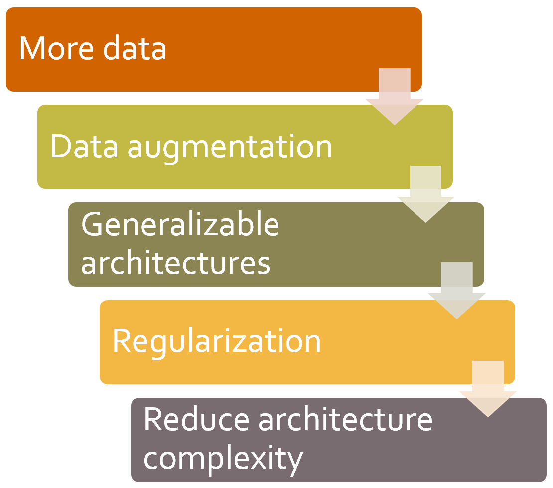
Many practitioners, when faced with an overfitting model, start at exactly the wrong end of this diagram. Their starting point is to use a smaller model, or more regularization. Using a smaller model should be absolutely the last step you take, unless training your model is taking up too much time or memory. Reducing the size of your model reduces the ability of your model to learn subtle relationships in your data.
Instead, your first step should be to seek to create more data. That could involve adding more labels to data that you already have, finding additional tasks that your model could be asked to solve (or, to think of it another way, identifying different kinds of labels that you could model), or creating additional synthetic data by using more or different data augmentation techniques. Thanks to the development of Mixup and similar approaches, effective data augmentation is now available for nearly all kinds of data.
Once you've got as much data as you think you can reasonably get hold of, and are using it as effectively as possible by taking advantage of all the labels that you can find and doing all the augmentation that makes sense, if you are still overfitting you should think about using more generalizable architectures. For instance, adding batch normalization may improve generalization.
If you are still overfitting after doing the best you can at using your data and tuning your architecture, then you can take a look at regularization. Generally speaking, adding dropout to the last layer or two will do a good job of regularizing your model. However, as we learned from the story of the development of AWD-LSTM, it is often the case that adding dropout of different types throughout your model can help even more. Generally speaking, a larger model with more regularization is more flexible, and can therefore be more accurate than a smaller model with less regularization.
Only after considering all of these options would we recommend that you try using a smaller version of your architecture.
许多从业者在面对过拟合模型时,会从该图的错误一端开始。他们的出发点是使用更小的模型,或者更多的正则化。使用较小的模型绝对应该是您采取的最后一步,除非训练您的模型占用太多时间或内存。减小模型的大小会降低模型学习数据中微妙关系的能力。
相反,您的第一步应该是寻求创建更多数据。这可能涉及为您已经拥有的数据添加更多标签,查找可能要求您的模型解决的其他任务(或者,换一种方式考虑,识别您可以建模的不同类型的标签),或创建额外的合成数据通过使用更多或不同的数据增强技术。由于 Mixup 和类似方法的发展,现在几乎所有类型的数据都可以使用有效的数据增强。
一旦您获得了您认为可以合理掌握的尽可能多的数据,并通过利用您可以找到的所有标签并进行所有有意义的增强,尽可能有效地使用它,如果您仍然过度拟合你应该考虑使用更通用的架构。例如,添加批量标准化可能会提高泛化能力。
如果您在尽最大努力使用数据和调整架构后仍然过拟合,那么您可以看看正则化。一般来说,在最后一两层添加 dropout 可以很好地规范你的模型。然而,正如我们从 AWD-LSTM 的发展故事中了解到的那样,通常情况下,在整个模型中添加不同类型的 dropout 可以提供更多帮助。一般来说,具有更多正则化的较大模型更灵活,因此可以比具有较少正则化的较小模型更准确。
只有在考虑了所有这些选项之后,我们才会建议您尝试使用较小版本的架构。
Questionnaire
- What is the "head" of a neural net?
- What is the "body" of a neural net?
- What is "cutting" a neural net? Why do we need to do this for transfer learning?
- What is
model_meta? Try printing it to see what's inside. - Read the source code for
create_headand make sure you understand what each line does. - Look at the output of
create_headand make sure you understand why each layer is there, and how thecreate_headsource created it. - Figure out how to change the dropout, layer size, and number of layers created by
vision_learner, and see if you can find values that result in better accuracy from the pet recognizer. - What does
AdaptiveConcatPool2ddo? - What is "nearest neighbor interpolation"? How can it be used to upsample convolutional activations?
- What is a "transposed convolution"? What is another name for it?
- Create a conv layer with
transpose=Trueand apply it to an image. Check the output shape. - Draw the U-Net architecture.
- What is "BPTT for Text Classification" (BPT3C)?
- How do we handle different length sequences in BPT3C?
- Try to run each line of
TabularModel.forwardseparately, one line per cell, in a notebook, and look at the input and output shapes at each step. - How is
self.layersdefined inTabularModel? - What are the five steps for preventing over-fitting?
- Why don't we reduce architecture complexity before trying other approaches to preventing overfitting?
Further Research
- Write your own custom head and try training the pet recognizer with it. See if you can get a better result than fastai's default.
- Try switching between
AdaptiveConcatPool2dandAdaptiveAvgPool2din a CNN head and see what difference it makes. - Write your own custom splitter to create a separate parameter group for every ResNet block, and a separate group for the stem. Try training with it, and see if it improves the pet recognizer.
- Read the online chapter about generative image models, and create your own colorizer, super-resolution model, or style transfer model.
- Create a custom head using nearest neighbor interpolation and use it to do segmentation on CamVid.