
Chapter 09
Tabular Modeling Deep Dive
#hide
! [ -e /content ] && pip install -Uqq fastbook kaggle waterfallcharts treeinterpreter dtreeviz
import fastbook
fastbook.setup_book()#hide
from fastbook import *
from pandas.api.types import is_string_dtype, is_numeric_dtype, is_categorical_dtype
from fastai.tabular.all import *
from sklearn.ensemble import RandomForestRegressor
from sklearn.tree import DecisionTreeRegressor
from dtreeviz.trees import *
from IPython.display import Image, display_svg, SVG
pd.options.display.max_rows = 20
pd.options.display.max_columns = 8Tabular Modeling Deep Dive
深入探讨表格建模
Tabular modeling takes data in the form of a table (like a spreadsheet or CSV). The objective is to predict the value in one column based on the values in the other columns. In this chapter we will not only look at deep learning but also more general machine learning techniques like random forests, as they can give better results depending on your problem.
We will look at how we should preprocess and clean the data as well as how to interpret the result of our models after training, but first, we will see how we can feed columns that contain categories into a model that expects numbers by using embeddings.
表格建模采用表格形式的数据(如电子表格或CSV)。目标是根据其他列中的值预测一列中的值。在这一章中,我们不仅会关注深度学习,还将关注更通用的机器学习技术,比如随机森林,因为它们可以根据你的问题给出更好的结果。
我们将研究如何预处理和清理数据,以及如何在训练后解释模型的结果,但首先,我们将看到如何通过使用嵌入将包含类别的列输入到期望数字的模型中。
Categorical Embeddings
分类嵌入
In tabular data some columns may contain numerical data, like "age," while others contain string values, like "sex." The numerical data can be directly fed to the model (with some optional preprocessing), but the other columns need to be converted to numbers. Since the values in those correspond to different categories, we often call this type of variables categorical variables. The first type are called continuous variables.
在表格数据中,一些列可能包含数值数据,如“年龄”,而另一些列可能包含字符串值,如“性别”。数值数据可以直接输入模型(通过一些可选的预处理),但其他列需要转换为数字。由于其中的值对应于不同的类别,我们通常将此类变量称为分类变量。第一类称为连续变量。
jargon: Continuous and Categorical Variables: Continuous variables are numerical data, such as "age," that can be directly fed to the model, since you can add and multiply them directly. Categorical variables contain a number of discrete levels, such as "movie ID," for which addition and multiplication don't have meaning (even if they're stored as numbers).
术语:连续变量和分类变量:连续变量是数值数据,比如“年龄”,可以直接输入到模型中,因为你可以直接将它们相加和相乘。分类变量包含许多离散的级别,例如“电影ID”,加法和乘法对其没有意义(即使它们以数字的形式存储)。
At the end of 2015, the Rossmann sales competition ran on Kaggle. Competitors were given a wide range of information about various stores in Germany, and were tasked with trying to predict sales on a number of days. The goal was to help the company to manage stock properly and be able to satisfy demand without holding unnecessary inventory. The official training set provided a lot of information about the stores. It was also permitted for competitors to use additional data, as long as that data was made public and available to all participants.
One of the gold medalists used deep learning, in one of the earliest known examples of a state-of-the-art deep learning tabular model. Their method involved far less feature engineering, based on domain knowledge, than those of the other gold medalists. The paper, "Entity Embeddings of Categorical Variables" describes their approach. In an online-only chapter on the book's website we show how to replicate it from scratch and attain the same accuracy shown in the paper. In the abstract of the paper the authors (Cheng Guo and Felix Berkhahn) say:
2015年底,Rossmann销售竞赛在Kaggle上进行。参赛者获得了德国各家商店的广泛信息,并被要求尝试预测几天内的销售情况。目标是帮助公司正确管理库存并能够在不持有不必要库存的情况下满足需求。官方训练集提供了大量关于商店的信息。参赛者也可以使用额外的数据,只要这些数据是公开的并对所有参赛者开放。
其中一位金牌得主使用了深度学习,这是已知最早的最先进的深度学习表格模型示例之一。与其他金牌得主相比,他们的方法涉及的基于领域知识的特征工程要少得多。论文“分类变量的实体嵌入”描述了他们的方法。在本书网站上仅在线的一章中,我们展示了如何从头开始复制它,并获得与论文中相同的精度。在论文摘要中,作者(Cheng Guo和Felix Berkhahn)说:
: Entity embedding not only reduces memory usage and speeds up neural networks compared with one-hot encoding, but more importantly by mapping similar values close to each other in the embedding space it reveals the intrinsic properties of the categorical variables... [It] is especially useful for datasets with lots of high cardinality features, where other methods tend to overfit... As entity embedding defines a distance measure for categorical variables it can be used for visualizing categorical data and for data clustering.
:与独热编码相比,实体嵌入不仅减少了内存的使用,加快了神经网络的速度,更重要的是,通过在嵌入空间中将相似的值映射到彼此靠近的位置,它揭示了分类变量的内在属性……[它]对于具有大量高基数特征的数据集特别有用,而其他方法往往会过度拟合……由于实体嵌入定义了分类变量的距离度量,它可用于可视化分类数据和数据聚类。
We have already noticed all of these points when we built our collaborative filtering model. We can clearly see that these insights go far beyond just collaborative filtering, however.
The paper also points out that (as we discussed in the last chapter) an embedding layer is exactly equivalent to placing an ordinary linear layer after every one-hot-encoded input layer. The authors used the diagram in <<entity_emb>> to show this equivalence. Note that "dense layer" is a term with the same meaning as "linear layer," and the one-hot encoding layers represent inputs.
当我们构建协同过滤模型时,我们已经注意到所有这些点。然而,我们可以清楚地看到,这些见解远远超出了协同过滤。
论文还指出(正如我们在上一章所讨论的)嵌入层完全等价于在每个独热编码输入层之后放置一个普通的线性层。作者使用<<entity_emb>>中的图表来显示这种等价性。请注意,“密集层”是一个与“线性层”含义相同的术语,独热编码层表示输入。
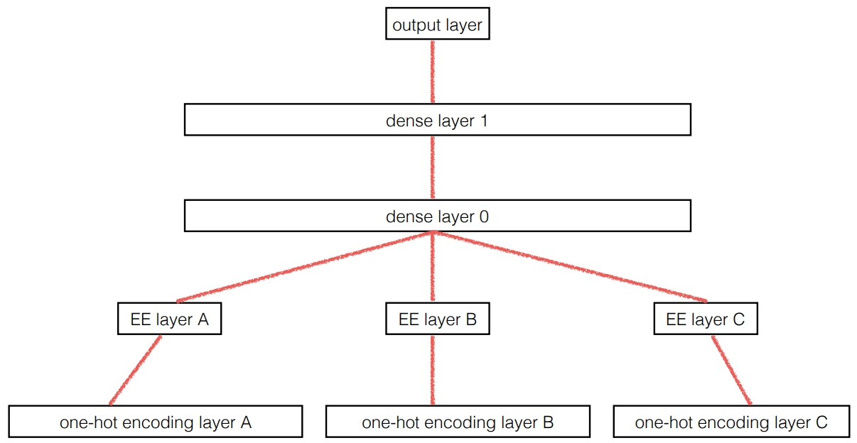
The insight is important because we already know how to train linear layers, so this shows that from the point of view of the architecture and our training algorithm the embedding layer is just another layer. We also saw this in practice in the last chapter, when we built a collaborative filtering neural network that looks exactly like this diagram.
Where we analyzed the embedding weights for movie reviews, the authors of the entity embeddings paper analyzed the embedding weights for their sales prediction model. What they found was quite amazing, and illustrates their second key insight. This is that the embedding transforms the categorical variables into inputs that are both continuous and meaningful.
The images in <<state_emb>> illustrate these ideas. They are based on the approaches used in the paper, along with some analysis we have added.
洞察力很重要,因为我们已经知道如何训练线性层,所以这表明,从架构和我们的训练算法的角度来看,嵌入层只是另一层。我们在上一章的实践中也看到了这一点,当时我们构建了一个看起来与此图完全相同的协同过滤神经网络。
在我们分析电影评论的嵌入权重时,实体嵌入论文的作者分析了他们的销售预测模型的嵌入权重。他们的发现非常惊人,也说明了他们的第二个关键见解。这是嵌入将分类变量转换为连续且有意义的输入。
<<state_emb>>中的图像说明了这些想法。它们基于论文中使用的方法,以及我们添加的一些分析。
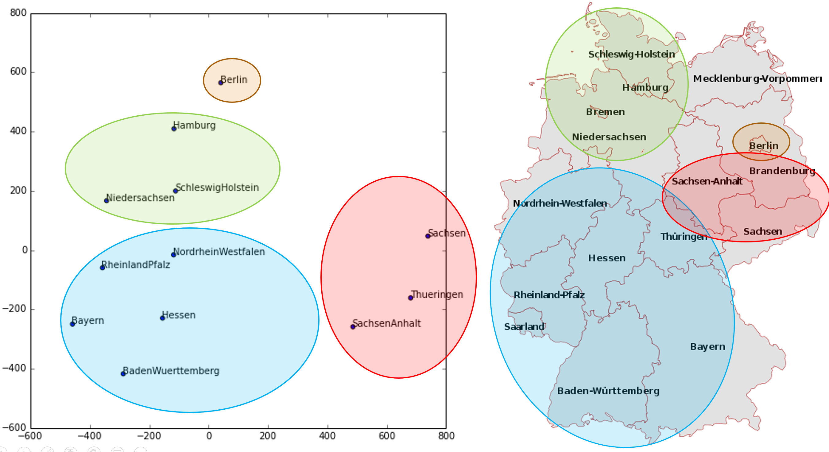
On the left is a plot of the embedding matrix for the possible values of the State category. For a categorical variable we call the possible values of the variable its "levels" (or "categories" or "classes"), so here one level is "Berlin," another is "Hamburg," etc. On the right is a map of Germany. The actual physical locations of the German states were not part of the provided data, yet the model itself learned where they must be, based only on the behavior of store sales!
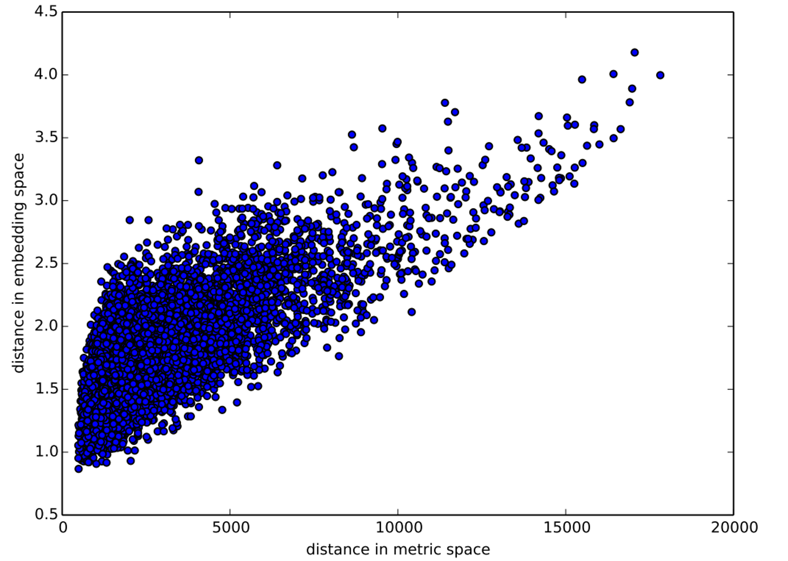
Do you remember how we talked about distance between embeddings? The authors of the paper plotted the distance between store embeddings against the actual geographic distance between the stores (see <<store_emb>>). They found that they matched very closely!
左边是State类别可能值的嵌入矩阵图。对于一个分类变量,我们称其可能的值为“级别”(或“类别”或“类”),所以这里一个级别是“柏林”,另一个级别是“汉堡”,等。右边是一张德国地图。德国各州的实际物理位置并不是所提供数据的一部分,但模型本身仅根据商店销售行为就知道它们必须在哪里!
还记得我们如何谈论嵌入之间的距离吗?这篇论文的作者绘制了商店嵌入之间的距离与商店之间的实际地理距离(参见<<store_emb>>)。他们发现他们非常匹配!
We've even tried plotting the embeddings for days of the week and months of the year, and found that days and months that are near each other on the calendar ended up close as embeddings too, as shown in <<date_emb>>.
我们甚至尝试绘制一周中的天数和一年中的月份的嵌入图,发现日历上彼此靠近的日期和月份最终也接近嵌入,如<<date_emb>>所示。
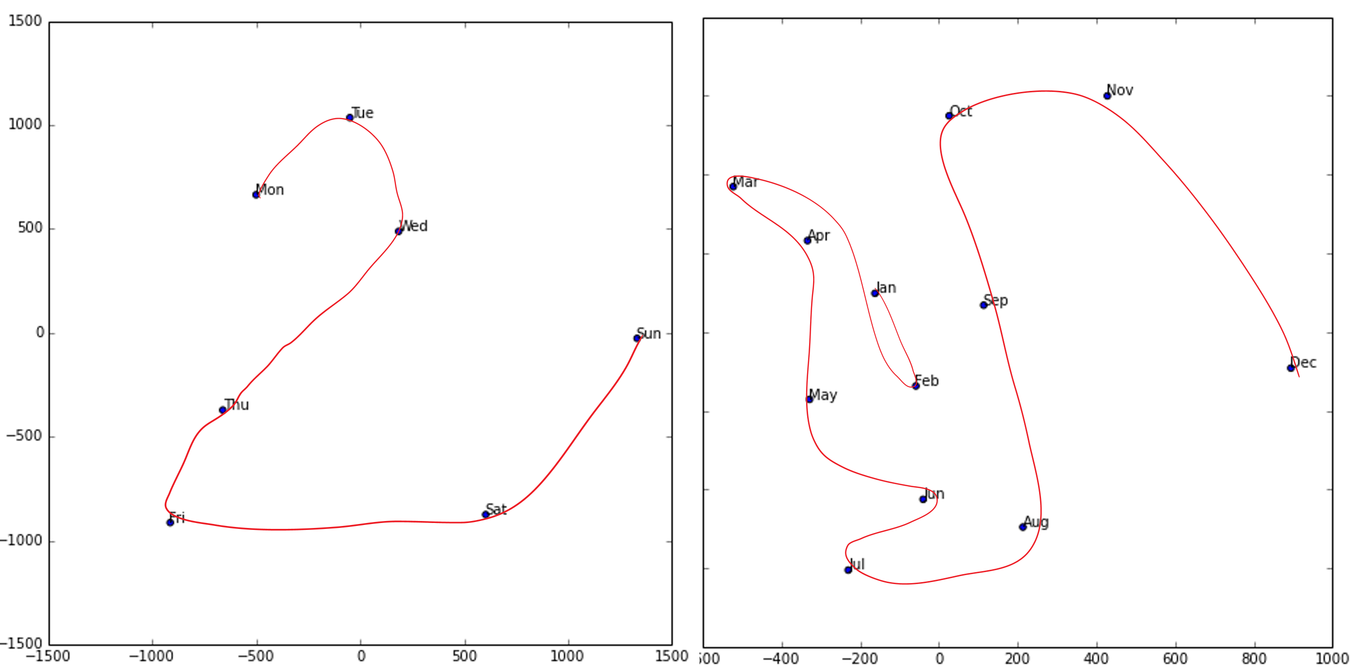
What stands out in these two examples is that we provide the model fundamentally categorical data about discrete entities (e.g., German states or days of the week), and then the model learns an embedding for these entities that defines a continuous notion of distance between them. Because the embedding distance was learned based on real patterns in the data, that distance tends to match up with our intuitions.
In addition, it is valuable in its own right that embeddings are continuous, because models are better at understanding continuous variables. This is unsurprising considering models are built of many continuous parameter weights and continuous activation values, which are updated via gradient descent (a learning algorithm for finding the minimums of continuous functions).
Another benefit is that we can combine our continuous embedding values with truly continuous input data in a straightforward manner: we just concatenate the variables, and feed the concatenation into our first dense layer. In other words, the raw categorical data is transformed by an embedding layer before it interacts with the raw continuous input data. This is how fastai and Guo and Berkhahn handle tabular models containing continuous and categorical variables.
An example using this concatenation approach is how Google does its recommendations on Google Play, as explained in the paper "Wide & Deep Learning for Recommender Systems". <<google_recsys>> illustrates.
这两个例子的突出之处在于,我们为模型提供了关于离散实体的基本分类数据(例如,德国各州或一周的天数),然后模型学习了这些实体的嵌入,定义了它们之间距离的连续概念。因为嵌入距离是根据数据中的真实模式学习的,所以该距离往往与我们的直觉相匹配。
此外,嵌入是连续的本身就很有价值,因为模型更擅长理解连续变量。这并不奇怪,因为模型是由许多连续参数权值和连续激活值构建的,这些值通过梯度下降(一种寻找连续函数最小值的学习算法)进行更新。
另一个好处是,我们可以以一种直接的方式将连续嵌入值与真正连续的输入数据结合起来:我们只是将变量连接起来,并将连接输入到我们的第一个密集层中。换句话说,原始分类数据在与原始连续输入数据交互之前先由嵌入层进行转换。这就是fastai、Guo和Berkhahn处理包含连续变量和分类变量的表格模型的方法。
使用这种连接方法的一个例子是Google如何在Google Play上进行推荐,正如论文推荐系统的广泛和深度学习中解释的那样。<<google_recsys>>说明。
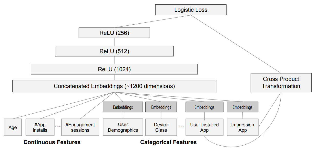
Interestingly, the Google team actually combined both approaches we saw in the previous chapter: the dot product (which they call cross product) and neural network approaches.
Let's pause for a moment. So far, the solution to all of our modeling problems has been: train a deep learning model. And indeed, that is a pretty good rule of thumb for complex unstructured data like images, sounds, natural language text, and so forth. Deep learning also works very well for collaborative filtering. But it is not always the best starting point for analyzing tabular data.
有趣的是,谷歌团队实际上结合了我们在上一章看到的两种方法:点积(他们称之为叉积)和神经网络方法。
让我们暂停一下。到目前为止,我们所有建模问题的解决方案都是:训练一个深度学习模型。事实上,对于图像、声音、自然语言文本等复杂的非结构化数据,这是一个非常好的经验法则。深度学习对于协同过滤也非常有效。但它并不总是分析表格数据的最佳起点。
Beyond Deep Learning
超越深度学习
Most machine learning courses will throw dozens of different algorithms at you, with a brief technical description of the math behind them and maybe a toy example. You're left confused by the enormous range of techniques shown and have little practical understanding of how to apply them.
The good news is that modern machine learning can be distilled down to a couple of key techniques that are widely applicable. Recent studies have shown that the vast majority of datasets can be best modeled with just two methods:
- Ensembles of decision trees (i.e., random forests and gradient boosting machines), mainly for structured data (such as you might find in a database table at most companies)
- Multilayered neural networks learned with SGD (i.e., shallow and/or deep learning), mainly for unstructured data (such as audio, images, and natural language)
大多数机器学习课程都会向你抛出几十种不同的算法,并对它们背后的数学进行简要的技术描述,也许还有一个玩具示例。您对所展示的大量技术感到困惑,并且对如何应用它们几乎没有实际的理解。
好消息是,现代机器学习可以提炼成几个广泛适用的关键技术。最近的研究表明,绝大多数数据集可以用两种方法进行最好的建模:
- 决策树的集合(即随机森林和梯度提升机),主要用于结构化数据(如您可能在大多数公司的数据库表中找到)
- 使用SGD学习的多层神经网络(即浅层和/或深度学习),主要用于非结构化数据(如音频、图像和自然语言)
Although deep learning is nearly always clearly superior for unstructured data, these two approaches tend to give quite similar results for many kinds of structured data. But ensembles of decision trees tend to train faster, are often easier to interpret, do not require special GPU hardware for inference at scale, and often require less hyperparameter tuning. They have also been popular for quite a lot longer than deep learning, so there is a more mature ecosystem of tooling and documentation around them.
Most importantly, the critical step of interpreting a model of tabular data is significantly easier for decision tree ensembles. There are tools and methods for answering the pertinent questions, like: Which columns in the dataset were the most important for your predictions? How are they related to the dependent variable? How do they interact with each other? And which particular features were most important for some particular observation?
Therefore, ensembles of decision trees are our first approach for analyzing a new tabular dataset.
The exception to this guideline is when the dataset meets one of these conditions:
- There are some high-cardinality categorical variables that are very important ("cardinality" refers to the number of discrete levels representing categories, so a high-cardinality categorical variable is something like a zip code, which can take on thousands of possible levels).
- There are some columns that contain data that would be best understood with a neural network, such as plain text data.
In practice, when we deal with datasets that meet these exceptional conditions, we always try both decision tree ensembles and deep learning to see which works best. It is likely that deep learning will be a useful approach in our example of collaborative filtering, as we have at least two high-cardinality categorical variables: the users and the movies. But in practice things tend to be less cut-and-dried, and there will often be a mixture of high- and low-cardinality categorical variables and continuous variables.
Either way, it's clear that we are going to need to add decision tree ensembles to our modeling toolbox!
尽管深度学习对于非结构化数据来说几乎总是明显更好,但这两种方法往往会对多种结构化数据产生非常相似的结果。但是决策树的集合往往训练得更快,通常更容易解释,不需要特殊的GPU硬件来进行大规模推理,通常需要较少的超参数调优。它们比深度学习流行的时间要长得多,因此围绕它们有一个更成熟的工具和文档生态系统。
最重要的是,解释表格数据模型的关键步骤对于决策树集成来说要容易的多。有一些工具和方法可以回答相关的问题,比如:数据集中哪些列对您的预测最重要?它们与因变量有什么关系?它们是如何相互作用的?哪些特定特征对某些特定观察最重要?
因此,决策树集成是我们分析新表格数据集的第一种方法。
本指南的例外情况是数据集满足以下条件之一:
- 有一些高基数的分类变量非常重要(“基数”指的是表示类别的离散级别的数量,所以高基数的分类变量就像邮政编码一样,可以有数千个可能的级别)。
- 有些列包含的数据最适合用神经网络来理解,比如纯文本数据。
在实践中,当我们处理满足这些特殊条件的数据集时,我们总是同时尝试决策树集成和深度学习,看看哪种效果最好。在我们的协同过滤示例中,深度学习很可能是一种有用的方法,因为我们至少有两个高基数的分类变量:用户和电影。但在实践中,事情往往不那么简单,通常会混合高基数和低基数的分类变量和连续变量。
无论哪种方式,很明显我们都需要将决策树集成添加到我们的建模工具箱中!
Up to now we've used PyTorch and fastai for pretty much all of our heavy lifting. But these libraries are mainly designed for algorithms that do lots of matrix multiplication and derivatives (that is, stuff like deep learning!). Decision trees don't depend on these operations at all, so PyTorch isn't much use.
Instead, we will be largely relying on a library called scikit-learn (also known as sklearn). Scikit-learn is a popular library for creating machine learning models, using approaches that are not covered by deep learning. In addition, we'll need to do some tabular data processing and querying, so we'll want to use the Pandas library. Finally, we'll also need NumPy, since that's the main numeric programming library that both sklearn and Pandas rely on.
We don't have time to do a deep dive into all these libraries in this book, so we'll just be touching on some of the main parts of each. For a far more in depth discussion, we strongly suggest Wes McKinney's Python for Data Analysis (O'Reilly). Wes is the creator of Pandas, so you can be sure that the information is accurate!
First, let's gather the data we will use.
到目前为止,我们已经使用PyTorch和fastai完成了几乎所有繁重的工作。但这些库主要是为做大量矩阵乘法和导数的算法设计的(也就是说,像深度学习这样的东西!)。决策树根本不依赖于这些操作,所以PyTorch用处不大。
相反,我们将在很大程度上依赖于一个叫做scikit-learn(也称为sklearn)的库。Scikit-learn是一个用于创建机器学习模型的流行库,使用深度学习未涵盖的方法。此外,我们需要进行一些表格数据处理和查询,因此我们需要使用Pandas库。最后,我们还需要NumPy,因为它是sklearn和Pandas都依赖的主要数字编程库。
我们没有时间深入探讨本书中的所有这些库,所以我们将只触及每个库的一些主要部分。要进行更深入的讨论,我们强烈推荐Wes McKinney的Python For Data Analysis (O'Reilly)。Wes是Pandas的创造者,所以你可以确定信息是准确的!
首先,让我们收集我们将使用的数据。
The Dataset
数据集
The dataset we use in this chapter is from the Blue Book for Bulldozers Kaggle competition, which has the following description: "The goal of the contest is to predict the sale price of a particular piece of heavy equipment at auction based on its usage, equipment type, and configuration. The data is sourced from auction result postings and includes information on usage and equipment configurations."
This is a very common type of dataset and prediction problem, similar to what you may see in your project or workplace. The dataset is available for download on Kaggle, a website that hosts data science competitions.
我们在本章中使用的数据集来自 Bulldozers Kaggle竞赛蓝皮书,其中有如下描述:“竞赛的目标是根据特定重型设备的使用情况、设备类型和配置,在拍卖中预测其销售价格。数据来自发布的拍卖结果,包括有关使用和设备配置的信息。”
这是一种非常常见的数据集和预测问题,类似于您在项目或工作场所中可能看到的问题。该数据集可在举办数据科学竞赛的网站Kaggle上下载。
Kaggle Competitions
Kaggle竞赛
Kaggle is an awesome resource for aspiring data scientists or anyone looking to improve their machine learning skills. There is nothing like getting hands-on practice and receiving real-time feedback to help you improve your skills.
Kaggle provides:
- Interesting datasets
- Feedback on how you're doing
- A leaderboard to see what's good, what's possible, and what's state-of-the-art
- Blog posts by winning contestants sharing useful tips and techniques
Until now all our datasets have been available to download through fastai's integrated dataset system. However, the dataset we will be using in this chapter is only available from Kaggle. Therefore, you will need to register on the site, then go to the page for the competition. On that page click "Rules," then "I Understand and Accept." (Although the competition has finished, and you will not be entering it, you still have to agree to the rules to be allowed to download the data.)
The easiest way to download Kaggle datasets is to use the Kaggle API. You can install this using pip by running this in a notebook cell:
!pip install kaggleYou need an API key to use the Kaggle API; to get one, click on your profile picture on the Kaggle website, and choose My Account, then click Create New API Token. This will save a file called kaggle.json to your PC. You need to copy this key on your GPU server. To do so, open the file you downloaded, copy the contents, and paste them in the following cell in the notebook associated with this chapter (e.g., creds = '{"username":"xxx","key":"xxx"}'):
对于有抱负的数据科学家或任何希望提高机器学习技能的人来说,Kaggle是一个很棒的资源。没有什么比动手实践和接收实时反馈更能帮助你提高技能了。
Kaggle提供:
- 有趣的数据集
- 对您的表现的反馈
- 一个排行榜,看看什么是好的,什么是可能的,什么是最先进的
- 获奖选手分享有用技巧和技术的博客文章
到目前为止,我们所有的数据集都可以通过fastai的集成数据集系统下载。但是,我们将在本章中使用的数据集只能从Kaggle获得。因此,你需要在网站上注册,然后进入比赛页面。在该页面上单击“规则”,然后点击“我理解并接受”。(虽然比赛已经结束,你不会参加,但你仍然必须同意规则,才能被允许下载数据。)
下载Kaggle数据集最简单的方法是使用Kaggle API。你可以通过在笔记本单元中运行pip来安装它:
!pip install kaggle你需要一个API密钥才能使用Kaggle API;要获得一个,请在Kaggle网站上单击您的个人资料图片,然后选择我的帐户,然后单击创建新的API令牌。这将保存一个名为kaggle.json的文件到您的PC。您需要在GPU服务器上复制此密钥。为此,请打开您下载的文件,复制内容,并将它们粘贴到与本章相关的笔记本中的以下单元格中(如,creds = '{"username":"xxx","key":"xxx"}'):
creds = ''Then execute this cell (this only needs to be run once):
然后执行这个单元格(这只需要运行一次):
cred_path = Path('~/.kaggle/kaggle.json').expanduser()
if not cred_path.exists():
    cred_path.parent.mkdir(exist_ok=True)
    cred_path.write_text(creds)
    cred_path.chmod(0o600)
Now you can download datasets from Kaggle! Pick a path to download the dataset to:
现在您可以从Kaggle下载数据集!选择将数据集下载到的路径:
comp = 'bluebook-for-bulldozers'
path = URLs.path(comp)
path
Output
Path('/home/jhoward/.fastai/archive/bluebook-for-bulldozers')#hide
Path.BASE_PATH = pathAnd use the Kaggle API to download the dataset to that path, and extract it:
并使用Kaggle API将数据集下载到该路径,并提取它:
from kaggle import api

if not path.exists():
    path.mkdir(parents=true)
    api.competition_download_cli(comp, path=path)
    shutil.unpack_archive(str(path/f'{comp}.zip'), str(path))

path.ls(file_type='text')
Output
(#7) [Path('ValidSolution.csv'),Path('Machine_Appendix.csv'),Path('TrainAndValid.csv'),Path('median_benchmark.csv'),Path('random_forest_benchmark_test.csv'),Path('Test.csv'),Path('Valid.csv')]Now that we have downloaded our dataset, let's take a look at it!
现在我们已经下载了我们的数据集,让我们来看看它!
Look at the Data
查看数据
Kaggle provides information about some of the fields of our dataset. The Data explains that the key fields in train.csv are:
SalesID:: The unique identifier of the sale.MachineID:: The unique identifier of a machine. A machine can be sold multiple times.saleprice:: What the machine sold for at auction (only provided in train.csv).saledate:: The date of the sale.
In any sort of data science work, it's important to look at your data directly to make sure you understand the format, how it's stored, what types of values it holds, etc. Even if you've read a description of the data, the actual data may not be what you expect. We'll start by reading the training set into a Pandas DataFrame. Generally it's a good idea to specify low_memory=False unless Pandas actually runs out of memory and returns an error. The low_memory parameter, which is True by default, tells Pandas to only look at a few rows of data at a time to figure out what type of data is in each column. This means that Pandas can actually end up using different data type for different rows, which generally leads to data processing errors or model training problems later.
Let's load our data and have a look at the columns:
Kaggle提供了有关我们数据集的一些字段的信息。数据解释了train.csv中的关键字段是:
SalesID::销售的唯一标识符。MachineID::机器的唯一标识符。一台机器可以多次出售。saleprice:机器在拍卖会上的售价(仅在train.csv中提供)。saledata:销售日期。
在任何类型的数据科学工作中,直接查看您的数据以确保您了解格式、存储方式、它包含哪些类型的值等都是很重要的。即使您已经阅读了数据的描述,实际数据也可能不是您所期望的。我们将从将训练集读入Pandas DataFrame开始。通常,指定low_memory=False是一个好主意,除非 Pandas 实际内存不足并返回错误。low_memory参数(默认为True)告诉Pandas每次只查看几行数据,以确定每列中的数据类型。这意味着Pandas实际上最终可能会对不同的行使用不同的数据类型,这通常会导致以后的数据处理错误或模型训练问题。
让我们加载数据并查看列:
df = pd.read_csv(path/'TrainAndValid.csv', low_memory=False)df.columnsOutput
Index(['SalesID', 'SalePrice', 'MachineID', 'ModelID', 'datasource',
       'auctioneerID', 'YearMade', 'MachineHoursCurrentMeter', 'UsageBand',
       'saledate', 'fiModelDesc', 'fiBaseModel', 'fiSecondaryDesc',
       'fiModelSeries', 'fiModelDescriptor', 'ProductSize',
       'fiProductClassDesc', 'state', 'ProductGroup', 'ProductGroupDesc',
       'Drive_System', 'Enclosure', 'Forks', 'Pad_Type', 'Ride_Control',
       'Stick', 'Transmission', 'Turbocharged', 'Blade_Extension',
       'Blade_Width', 'Enclosure_Type', 'Engine_Horsepower', 'Hydraulics',
       'Pushblock', 'Ripper', 'Scarifier', 'Tip_Control', 'Tire_Size',
       'Coupler', 'Coupler_System', 'Grouser_Tracks', 'Hydraulics_Flow',
       'Track_Type', 'Undercarriage_Pad_Width', 'Stick_Length', 'Thumb',
       'Pattern_Changer', 'Grouser_Type', 'Backhoe_Mounting', 'Blade_Type',
       'Travel_Controls', 'Differential_Type', 'Steering_Controls'],
      dtype='object')
That's a lot of columns for us to look at! Try looking through the dataset to get a sense of what kind of information is in each one. We'll shortly see how to "zero in" on the most interesting bits.
At this point, a good next step is to handle ordinal columns. This refers to columns containing strings or similar, but where those strings have a natural ordering. For instance, here are the levels of ProductSize:
我们要看很多列!试着浏览数据集以了解每个数据集包含哪些类型的信息。我们很快就会看到如何“归零”最有趣的部分。
现在,一个好的下一步是处理序数列。这是指包含字符串或类似内容的列,但这些字符串具有自然顺序。例如,以下是ProductSize的级别:
df['ProductSize'].unique()Output
array([nan, 'Medium', 'Small', 'Large / Medium', 'Mini', 'Large', 'Compact'], dtype=object)
We can tell Pandas about a suitable ordering of these levels like so:
我们可以告诉Pandas这些级别的合适顺序如下:
sizes = 'Large','Large / Medium','Medium','Small','Mini','Compact'df['ProductSize'] = df['ProductSize'].astype('category')
df['ProductSize'].cat.set_categories(sizes, ordered=True, inplace=True)The most important data column is the dependent variable—that is, the one we want to predict. Recall that a model's metric is a function that reflects how good the predictions are. It's important to note what metric is being used for a project. Generally, selecting the metric is an important part of the project setup. In many cases, choosing a good metric will require more than just selecting a variable that already exists. It is more like a design process. You should think carefully about which metric, or set of metrics, actually measures the notion of model quality that matters to you. If no variable represents that metric, you should see if you can build the metric from the variables that are available.
However, in this case Kaggle tells us what metric to use: root mean squared log error (RMSLE) between the actual and predicted auction prices. We need do only a small amount of processing to use this: we take the log of the prices, so that rmse of that value will give us what we ultimately need:
最重要的数据列是因变量——也就是我们想要预测的变量。回想一下,模型的指标是反映预测有多好的函数。重要的是要注意项目使用的指标。通常,选择指标是项目设置的重要组成部分。在许多情况下,选择一个好的指标需要的不仅仅是选择一个已经存在的变量。它更像是一个设计过程。您应该仔细考虑哪个指标,或一组指标,实际上衡量了对您很重要的模型质量的概念。如果没有变量表示该指标,您应该看看是否可以从可用的变量构建指标。
然而,在这种情况下,Kaggle告诉我们使用什么指标:实际和预测拍卖价格之间的均方根对数误差(RMSLE)。我们只需要做少量的处理即可使用它:我们取价格的对数,以便该值的rmse将为我们提供我们最终需要的:
dep_var = 'SalePrice'df[dep_var] = np.log(df[dep_var])We are now ready to explore our first machine learning algorithm for tabular data: decision trees.
现在我们准备探索我们的第一个表格数据机器学习算法:决策树。
Decision Trees
决策树
Decision tree ensembles, as the name suggests, rely on decision trees. So let's start there! A decision tree asks a series of binary (that is, yes or no) questions about the data. After each question the data at that part of the tree is split between a "yes" and a "no" branch, as shown in <<decision_tree>>. After one or more questions, either a prediction can be made on the basis of all previous answers or another question is required.
顾名思义,决策树集成依赖于决策树。所以让我们从那里开始!决策树询问一系列关于数据的二元(即是或否)问题。在每个问题之后,树中该部分的数据被分为“是”和“否”分支,如<<decision_tree>>所示。在一个或多个问题之后,要么根据之前所有的答案做出预测,要么需要另一个问题。
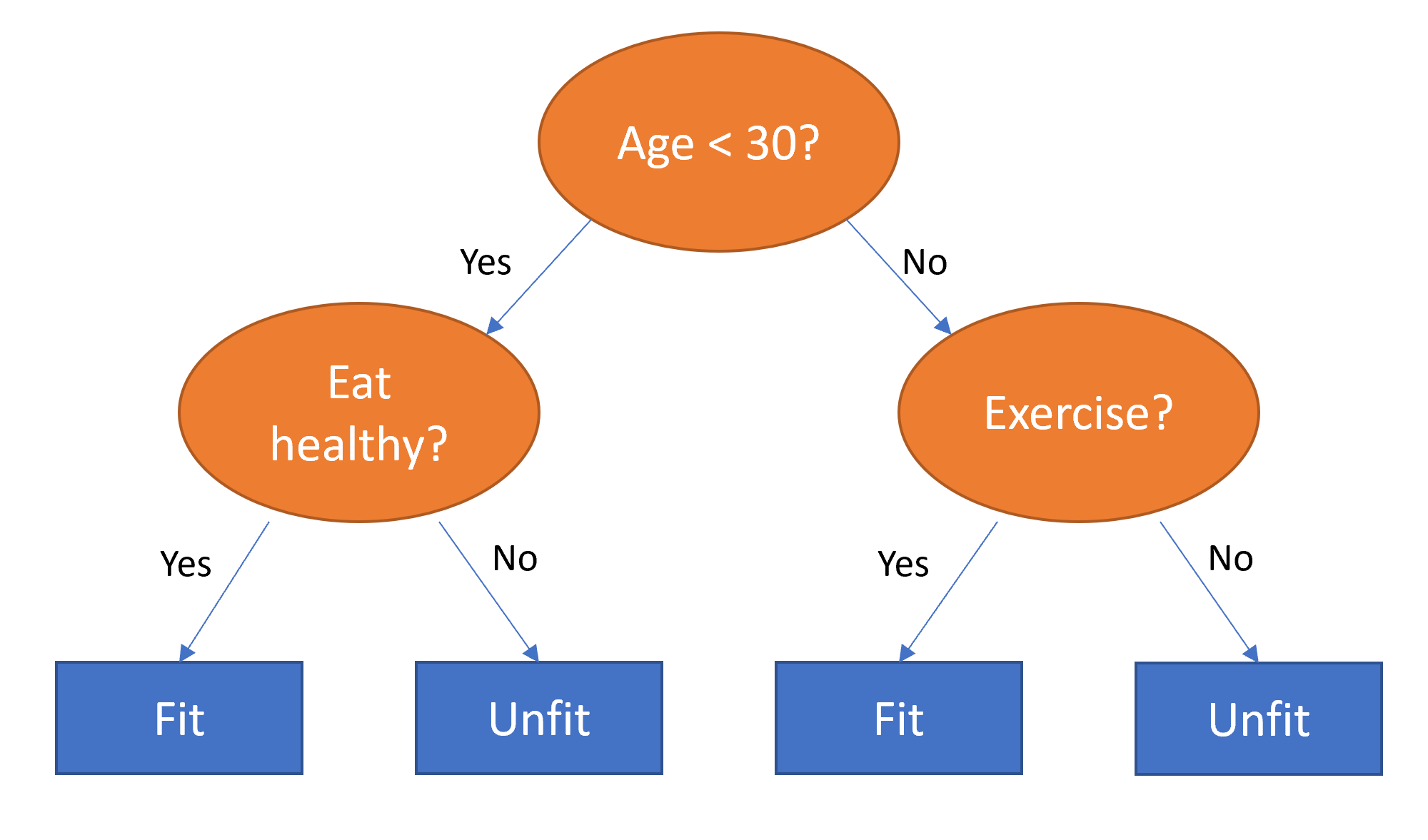
This sequence of questions is now a procedure for taking any data item, whether an item from the training set or a new one, and assigning that item to a group. Namely, after asking and answering the questions, we can say the item belongs to the same group as all the other training data items that yielded the same set of answers to the questions. But what good is this? The goal of our model is to predict values for items, not to assign them into groups from the training dataset. The value is that we can now assign a prediction value for each of these groups—for regression, we take the target mean of the items in the group.
Let's consider how we find the right questions to ask. Of course, we wouldn't want to have to create all these questions ourselves—that's what computers are for! The basic steps to train a decision tree can be written down very easily:
- Loop through each column of the dataset in turn.
- For each column, loop through each possible level of that column in turn.
- Try splitting the data into two groups, based on whether they are greater than or less than that value (or if it is a categorical variable, based on whether they are equal to or not equal to that level of that categorical variable).
- Find the average sale price for each of those two groups, and see how close that is to the actual sale price of each of the items of equipment in that group. That is, treat this as a very simple "model" where our predictions are simply the average sale price of the item's group.
- After looping through all of the columns and all the possible levels for each, pick the split point that gave the best predictions using that simple model.
- We now have two different groups for our data, based on this selected split. Treat each of these as separate datasets, and find the best split for each by going back to step 1 for each group.
- Continue this process recursively, until you have reached some stopping criterion for each group—for instance, stop splitting a group further when it has only 20 items in it.
Although this is an easy enough algorithm to implement yourself (and it is a good exercise to do so), we can save some time by using the implementation built into sklearn.
First, however, we need to do a little data preparation.
这个问题序列现在是一个程序,用于获取任何数据项,无论是来自训练集的项目还是新项目,并将该项目分配给一个组。也就是说,在提问和回答问题之后,我们可以说该项目与所有产生相同问题答案集的其他训练数据项目属于同一组。但这有什么好处呢?我们模型的目标是预测项目的值,而不是将它们从训练数据集分配到组中。价值在于我们现在可以为这些组中的每一个分配一个预测值——对于回归,我们取组中项目的目标平均值。
让我们考虑如何找到要问的正确问题。当然,我们不想自己制造所有这些问题——这就是计算机的作用!训练决策树的基本步骤可以很容易地写下来:
- 依次循环遍历数据集的每一列。
- 对于每一列,依次循环遍历该列的每个可能级别。
- 尝试将数据分成两组,基于它们是否大于或小于该值(或者如果它是分类变量,则基于它们是否等于或不等于该分类变量的该级别)。
- 找到这两组中每一组的平均销售价格,看看它与该组中每一件设备的实际销售价格有多接近。也就是说,将其视为一个非常简单的“模型”,我们的预测只是商品组的平均销售价格。
- 在遍历所有列和每个列的所有可能级别之后,选择使用该简单模型给出最佳预测的分割点。
- 基于这个选定的拆分,我们现在有两个不同的数据组。将每个数据集视为单独的数据集,并通过返回每个组的步骤1来找到每个组的最佳拆分。
- 递归地继续这个过程,直到每个组都达到某个停止标准——例如,当组中有20个项目时,停止进一步拆分。
尽管这是一个很容易自己实现的算法(而且是一个很好的练习),但我们可以通过使用sklearn中内置的实现来节省一些时间。
然而,首先我们需要做一些数据准备。
A: Here's a productive question to ponder. If you consider that the procedure for defining a decision tree essentially chooses one sequence of splitting questions about variables, you might ask yourself, how do we know this procedure chooses the correct sequence? The rule is to choose the splitting question that produces the best split (i.e., that most accurately separates the items into two distinct categories), and then to apply the same rule to the groups that split produces, and so on. This is known in computer science as a "greedy" approach. Can you imagine a scenario in which asking a “less powerful” splitting question would enable a better split down the road (or should I say down the trunk!) and lead to a better result overall?
A:这是一个值得深思的问题。如果你认为定义决策树的过程本质上选择了一个 关于变量的拆分问题序列 ,你可能会问自己,我们怎么知道这个过程选择了 正确的序列 ?规则是选择产生最佳拆分的拆分问题(即,最准确地将项目分成两个不同的类别),然后将相同的规则应用于拆分产生的组,以此类推。这在计算机科学中被称为“贪婪”方法。你能想象这样一种场景吗,问一个“不太强大”的拆分问题可以在未来更好地拆分(或者我应该说拆分主干!)并带来更好的整体结果?
Handling Dates
处理日期
The first piece of data preparation we need to do is to enrich our representation of dates. The fundamental basis of the decision tree that we just described is bisection— dividing a group into two. We look at the ordinal variables and divide up the dataset based on whether the variable's value is greater (or lower) than a threshold, and we look at the categorical variables and divide up the dataset based on whether the variable's level is a particular level. So this algorithm has a way of dividing up the dataset based on both ordinal and categorical data.
But how does this apply to a common data type, the date? You might want to treat a date as an ordinal value, because it is meaningful to say that one date is greater than another. However, dates are a bit different from most ordinal values in that some dates are qualitatively different from others in a way that that is often relevant to the systems we are modeling.
In order to help our algorithm handle dates intelligently, we'd like our model to know more than whether a date is more recent or less recent than another. We might want our model to make decisions based on that date's day of the week, on whether a day is a holiday, on what month it is in, and so forth. To do this, we replace every date column with a set of date metadata columns, such as holiday, day of week, and month. These columns provide categorical data that we suspect will be useful.
fastai comes with a function that will do this for us—we just have to pass a column name that contains dates:
我们需要做的第一件数据准备工作是丰富我们对日期的表示。我们刚才描述的决策树的基本原理是二分法——将一组分成两部分。我们查看序数变量,并根据变量的值是否大于(或低于)阈值来划分数据集,我们查看分类变量,并根据变量的级别是否为特定级别来划分数据集。因此,该算法有一种基于序数和分类数据来划分数据集的方法。
但是这如何应用于常见的数据类型,日期?您可能希望将日期视为序数值,因为说一个日期大于另一个日期是有意义的。然而,日期与大多数序数值有点不同,因为某些日期在质量上与其他日期不同,这通常与我们正在建模的系统有关。
为了帮助我们的算法智能地处理日期,我们希望我们的模型不仅仅知道一个日期是比另一个日期更近还是更远。我们可能希望我们的模型根据该日期是星期几、某一天是否是假期、它在哪个月等等做出决定。为此,我们将每个日期列替换为一组日期元数据列,如假期、星期几和月份。这些列提供了我们认为有用的分类数据。
fastai有一个函数可以为我们做到这一点——我们只需要传递一个包含日期的列名:
df = add_datepart(df, 'saledate')Let's do the same for the test set while we're there:
让我们在那里对测试集做同样的事情:
df_test = pd.read_csv(path/'Test.csv', low_memory=False)
df_test = add_datepart(df_test, 'saledate')
We can see that there are now lots of new columns in our DataFrame:
我们可以看到现在在我们的DataFrame中有很多新列:
' '.join(o for o in df.columns if o.startswith('sale'))Output
'saleWeek saleYear saleMonth saleDay saleDayofweek saleDayofyear saleIs_month_end saleIs_month_start saleIs_quarter_end saleIs_quarter_start saleIs_year_end saleIs_year_start saleElapsed'
This is a good first step, but we will need to do a bit more cleaning. For this, we will use fastai objects called TabularPandas and TabularProc.
这是很好的第一步,但我们需要做更多的清理。为此,我们将使用名为TabularPandas和TabularProc的fastai对象。
Using TabularPandas and TabularProc
使用TabularPandas和TabularProc
A second piece of preparatory processing is to be sure we can handle strings and missing data. Out of the box, sklearn cannot do either. Instead we will use fastai's class TabularPandas, which wraps a Pandas DataFrame and provides a few conveniences. To populate a TabularPandas, we will use two TabularProcs, Categorify and FillMissing. A TabularProc is like a regular Transform, except that:
- It returns the exact same object that's passed to it, after modifying the object in place.
- It runs the transform once, when data is first passed in, rather than lazily as the data is accessed.
Categorify is a TabularProc that replaces a column with a numeric categorical column. FillMissing is a TabularProc that replaces missing values with the median of the column, and creates a new Boolean column that is set to True for any row where the value was missing. These two transforms are needed for nearly every tabular dataset you will use, so this is a good starting point for your data processing:
准备处理的第二个部分是确保我们可以处理字符串和丢失的数据。开箱即用,sklearn也无法做到这一点。相反,我们将使用fastai的类TabularPandas,它包装了Pandas DataFrame,并提供了一些便利。要填充TabularPandas,我们将使用两个TabularProc, Categorify和FillMissing。TabularProc就像一个常规的Transform,除了:
- 在适当地修改对象后,它返回传递给它的完全相同的对象。
- 它在第一次传入数据时运行一次转换,而不是在访问数据时延迟运行。
Categorify是一个用数字分类列替换列的TabularProc。FillMissing是一个TabularProc,它用列的中位数替换缺失值,并为缺失值的任何行创建一个设置为True的新的布尔列。几乎您将使用的每个表格数据集都需要这两种转换,因此这是您数据处理的良好起点:
procs = [Categorify, FillMissing]TabularPandas will also handle splitting the dataset into training and validation sets for us. However we need to be very careful about our validation set. We want to design it so that it is like the test set Kaggle will use to judge the contest.
Recall the distinction between a validation set and a test set, as discussed in <<chapter_intro>>. A validation set is data we hold back from training in order to ensure that the training process does not overfit on the training data. A test set is data that is held back even more deeply, from us ourselves, in order to ensure that we don't overfit on the validation data, as we explore various model architectures and hyperparameters.
We don't get to see the test set. But we do want to define our validation data so that it has the same sort of relationship to the training data as the test set will have.
In some cases, just randomly choosing a subset of your data points will do that. This is not one of those cases, because it is a time series.
If you look at the date range represented in the test set, you will discover that it covers a six-month period from May 2012, which is later in time than any date in the training set. This is a good design, because the competition sponsor will want to ensure that a model is able to predict the future. But it means that if we are going to have a useful validation set, we also want the validation set to be later in time than the training set. The Kaggle training data ends in April 2012, so we will define a narrower training dataset which consists only of the Kaggle training data from before November 2011, and we'll define a validation set consisting of data from after November 2011.
To do this we use np.where, a useful function that returns (as the first element of a tuple) the indices of all True values:
TabularPandas还将为我们处理将数据集拆分成训练集和验证集。但是,我们需要非常小心我们的验证集。我们想把它设计成类似于Kaggle用来评判比赛的测试集。
回想一下验证集和测试集之间的区别,如<<chapter_intro>>中所讨论的。验证集是我们从训练中保留的数据,以确保训练过程不会过度拟合训练数据。测试集是我们自己保留的更深的数据,以确保我们在探索各种模型架构和超参数时不会过度拟合验证数据。
我们看不到测试集。但是我们确实希望定义我们的验证数据,以便它与训练数据具有与测试集相同的关系。
在某些情况下,只需随机选择数据点的子集就可以做到这一点。这不是其中一种情况,因为它是一个时间序列。
如果你查看测试集中表示的日期范围,你会发现它涵盖了从2012年5月开始的6个月的时间,这比训练集中的任何日期都晚。这是一个很好的设计,因为比赛赞助商希望确保一个模型能够预测未来。但这意味着,如果我们要有一个有用的验证集,我们也希望验证集在时间上比训练集晚。Kaggle训练数据将于2012年4月结束,因此我们将定义一个更窄的训练数据集,它只包含2011年11月之前的Kaggle训练数据,我们将定义一个由2011年11月之后的数据组成的验证集。
为此,我们使用np.where,这是一个有用的函数,它返回(作为元组的第一个元素)所有True值的索引:
cond = (df.saleYear<2011) | (df.saleMonth<10)
train_idx = np.where( cond)[0]
valid_idx = np.where(~cond)[0]

splits = (list(train_idx),list(valid_idx))
TabularPandas needs to be told which columns are continuous and which are categorical. We can handle that automatically using the helper function cont_cat_split:
需要告知TabularPandas哪些列是连续的,哪些列是分类的。我们可以使用辅助函数cont_cat_split来自动处理:
cont,cat = cont_cat_split(df, 1, dep_var=dep_var)to = TabularPandas(df, procs, cat, cont, y_names=dep_var, splits=splits)A TabularPandas behaves a lot like a fastai Datasets object, including providing train and valid attributes:
TabularPandas的行为很像fastai Datasets对象,包括提供train和valid的属性:
len(to.train),len(to.valid)Output
(404710, 7988)
We can see that the data is still displayed as strings for categories (we only show a few columns here because the full table is too big to fit on a page):
我们可以看到数据仍然显示为类别的字符串(我们在这里只显示几列,因为整个表格太大而无法放在页面上):
#hide_output
to.show(3)
Output
<IPython.core.display.HTML object>
| saleWeek | UsageBand | fiModelDesc | fiBaseModel | fiSecondaryDesc | fiModelSeries | fiModelDescriptor | ProductSize | fiProductClassDesc | state | ProductGroup | ProductGroupDesc | Drive_System | Enclosure | Forks | Pad_Type | Ride_Control | Stick | Transmission | Turbocharged | Blade_Extension | Blade_Width | Enclosure_Type | Engine_Horsepower | Hydraulics | Pushblock | Ripper | Scarifier | Tip_Control | Tire_Size | Coupler | Coupler_System | Grouser_Tracks | Hydraulics_Flow | Track_Type | Undercarriage_Pad_Width | Stick_Length | Thumb | Pattern_Changer | Grouser_Type | Backhoe_Mounting | Blade_Type | Travel_Controls | Differential_Type | Steering_Controls | saleIs_month_end | saleIs_month_start | saleIs_quarter_end | saleIs_quarter_start | saleIs_year_end | saleIs_year_start | saleElapsed | auctioneerID_na | MachineHoursCurrentMeter_na | SalesID | MachineID | ModelID | datasource | auctioneerID | YearMade | MachineHoursCurrentMeter | saleYear | saleMonth | saleDay | saleDayofweek | saleDayofyear | SalePrice | |
|---|---|---|---|---|---|---|---|---|---|---|---|---|---|---|---|---|---|---|---|---|---|---|---|---|---|---|---|---|---|---|---|---|---|---|---|---|---|---|---|---|---|---|---|---|---|---|---|---|---|---|---|---|---|---|---|---|---|---|---|---|---|---|---|---|---|---|---|
| 0 | 46 | Low | 521D | 521 | D | #na# | #na# | #na# | Wheel Loader - 110.0 to 120.0 Horsepower | Alabama | WL | Wheel Loader | #na# | EROPS w AC | None or Unspecified | #na# | None or Unspecified | #na# | #na# | #na# | #na# | #na# | #na# | #na# | 2 Valve | #na# | #na# | #na# | #na# | None or Unspecified | None or Unspecified | #na# | #na# | #na# | #na# | #na# | #na# | #na# | #na# | #na# | #na# | #na# | #na# | Standard | Conventional | False | False | False | False | False | False | 1163635200 | False | False | 1139246 | 999089 | 3157 | 121 | 3.0 | 2004 | 68.0 | 2006 | 11 | 16 | 3 | 320 | 11.097410 |
| 1 | 13 | Low | 950FII | 950 | F | II | #na# | Medium | Wheel Loader - 150.0 to 175.0 Horsepower | North Carolina | WL | Wheel Loader | #na# | EROPS w AC | None or Unspecified | #na# | None or Unspecified | #na# | #na# | #na# | #na# | #na# | #na# | #na# | 2 Valve | #na# | #na# | #na# | #na# | 23.5 | None or Unspecified | #na# | #na# | #na# | #na# | #na# | #na# | #na# | #na# | #na# | #na# | #na# | #na# | Standard | Conventional | False | False | False | False | False | False | 1080259200 | False | False | 1139248 | 117657 | 77 | 121 | 3.0 | 1996 | 4640.0 | 2004 | 3 | 26 | 4 | 86 | 10.950807 |
| 2 | 9 | High | 226 | 226 | #na# | #na# | #na# | #na# | Skid Steer Loader - 1351.0 to 1601.0 Lb Operating Capacity | New York | SSL | Skid Steer Loaders | #na# | OROPS | None or Unspecified | #na# | #na# | #na# | #na# | #na# | #na# | #na# | #na# | #na# | Auxiliary | #na# | #na# | #na# | #na# | #na# | None or Unspecified | None or Unspecified | None or Unspecified | Standard | #na# | #na# | #na# | #na# | #na# | #na# | #na# | #na# | #na# | #na# | #na# | False | False | False | False | False | False | 1077753600 | False | False | 1139249 | 434808 | 7009 | 121 | 3.0 | 2001 | 2838.0 | 2004 | 2 | 26 | 3 | 57 | 9.210340 |
#hide_input
to1 = TabularPandas(df, procs, ['state', 'ProductGroup', 'Drive_System', 'Enclosure'], [], y_names=dep_var, splits=splits)
to1.show(3)
Output
<IPython.core.display.HTML object>
| state | ProductGroup | Drive_System | Enclosure | SalePrice | |
|---|---|---|---|---|---|
| 0 | Alabama | WL | #na# | EROPS w AC | 11.097410 |
| 1 | North Carolina | WL | #na# | EROPS w AC | 10.950807 |
| 2 | New York | SSL | #na# | OROPS | 9.210340 |
However, the underlying items are all numeric:
但是,基础项都是数字:
#hide_output
to.items.head(3)
Output
   SalesID  SalePrice  MachineID  saleWeek  ...  saleIs_year_start  \
0  1139246  11.097410     999089        46  ...                  1
1  1139248  10.950807     117657        13  ...                  1
2  1139249   9.210340     434808         9  ...                  1

   saleElapsed  auctioneerID_na  MachineHoursCurrentMeter_na
0         2647                1                            1
1         2148                1                            1
2         2131                1                            1

[3 rows x 67 columns]
| SalesID | SalePrice | MachineID | saleWeek | ... | saleIs_year_start | saleElapsed | auctioneerID_na | MachineHoursCurrentMeter_na | |
|---|---|---|---|---|---|---|---|---|---|
| 0 | 1139246 | 11.097410 | 999089 | 46 | ... | 1 | 2647 | 1 | 1 |
| 1 | 1139248 | 10.950807 | 117657 | 13 | ... | 1 | 2148 | 1 | 1 |
| 2 | 1139249 | 9.210340 | 434808 | 9 | ... | 1 | 2131 | 1 | 1 |
3 rows × 67 columns
#hide_input
to1.items[['state', 'ProductGroup', 'Drive_System', 'Enclosure']].head(3)
Output
   state  ProductGroup  Drive_System  Enclosure
0      1             6             0          3
1     33             6             0          3
2     32             3             0          6
| state | ProductGroup | Drive_System | Enclosure | |
|---|---|---|---|---|
| 0 | 1 | 6 | 0 | 3 |
| 1 | 33 | 6 | 0 | 3 |
| 2 | 32 | 3 | 0 | 6 |
The conversion of categorical columns to numbers is done by simply replacing each unique level with a number. The numbers associated with the levels are chosen consecutively as they are seen in a column, so there's no particular meaning to the numbers in categorical columns after conversion. The exception is if you first convert a column to a Pandas ordered category (as we did for ProductSize earlier), in which case the ordering you chose is used. We can see the mapping by looking at the classes attribute:
将分类列转换为数字是通过简单地将每个唯一级别替换为一个数字来完成的。与级别相关的数字是连续选择的,因为它们在列中显示,所以转换后分类列中的数字没有特殊含义。例外情况是,如果您首先将列转换为Pandas排序类别(就像我们之前对ProductSize所做的那样),在这种情况下,将使用您选择的排序。我们可以通过查看classes属性来查看映射:
to.classes['ProductSize']Output
['#na#', 'Large', 'Large / Medium', 'Medium', 'Small', 'Mini', 'Compact']
Since it takes a minute or so to process the data to get to this point, we should save it—that way in the future we can continue our work from here without rerunning the previous steps. fastai provides a save method that uses Python's pickle system to save nearly any Python object:
由于处理数据需要一分钟左右的时间才能到达这一点,我们应该保存它——这样将来我们就可以从这里继续我们的工作,而无需重新运行前面的步骤。fastai提供了一个save方法,它使用Python的pickle系统来保存几乎任何Python对象:
save_pickle(path/'to.pkl',to)To read this back later, you would type:
to = (path/'to.pkl').load()稍后要阅读此内容,您可以输入:
to = (path/'to.pkl').load()Now that all this preprocessing is done, we are ready to create a decision tree.
现在所有这些预处理都完成了,我们准备创建一个决策树。
Creating the Decision Tree
创建决策树
To begin, we define our independent and dependent variables:
首先,我们定义自变量和因变量:
#hide
to = load_pickle(path/'to.pkl')xs,y = to.train.xs,to.train.y
valid_xs,valid_y = to.valid.xs,to.valid.yNow that our data is all numeric, and there are no missing values, we can create a decision tree:
现在我们的数据都是数字,并且没有缺失值,我们可以创建一个决策树:
m = DecisionTreeRegressor(max_leaf_nodes=4)
m.fit(xs, y);
To keep it simple, we've told sklearn to just create four leaf nodes. To see what it's learned, we can display the tree:
为了简单起见,我们告诉sklearn只创建四个叶节点。要查看它学到了什么,我们可以显示树:
draw_tree(m, xs, size=10, leaves_parallel=True, precision=2)Output
<graphviz.files.Source at 0x7fee5c5f8690>
%0A%20--%3E%0A%3C!--%20Title%3A%20Tree%20Pages%3A%201%20--%3E%0A%3Csvg%20width%3D%22629pt%22%20height%3D%22381pt%22%0A%20viewBox%3D%220.00%200.00%20628.56%20380.50%22%20xmlns%3D%22http%3A%2F%2Fwww.w3.org%2F2000%2Fsvg%22%20xmlns%3Axlink%3D%22http%3A%2F%2Fwww.w3.org%2F1999%2Fxlink%22%3E%0A%3Cg%20id%3D%22graph0%22%20class%3D%22graph%22%20transform%3D%22scale(1%201)%20rotate(0)%20translate(4%20376.5)%22%3E%0A%3Ctitle%3ETree%3C%2Ftitle%3E%0A%3Cpolygon%20fill%3D%22white%22%20stroke%3D%22transparent%22%20points%3D%22-4%2C4%20-4%2C-376.5%20624.56%2C-376.5%20624.56%2C4%20-4%2C4%22%2F%3E%0A%3C!--%200%20--%3E%0A%3Cg%20id%3D%22node1%22%20class%3D%22node%22%3E%0A%3Ctitle%3E0%3C%2Ftitle%3E%0A%3Cpath%20fill%3D%22%23eda775%22%20stroke%3D%22black%22%20d%3D%22M536.14%2C-373C536.14%2C-373%20409.14%2C-373%20409.14%2C-373%20403.14%2C-373%20397.14%2C-367%20397.14%2C-361%20397.14%2C-361%20397.14%2C-317%20397.14%2C-317%20397.14%2C-311%20403.14%2C-305%20409.14%2C-305%20409.14%2C-305%20536.14%2C-305%20536.14%2C-305%20542.14%2C-305%20548.14%2C-311%20548.14%2C-317%20548.14%2C-317%20548.14%2C-361%20548.14%2C-361%20548.14%2C-367%20542.14%2C-373%20536.14%2C-373%22%2F%3E%0A%3Ctext%20text-anchor%3D%22start%22%20x%3D%22405.14%22%20y%3D%22-357.8%22%20font-family%3D%22Helvetica%2Csans-Serif%22%20font-size%3D%2214.00%22%3ECoupler_System%20%E2%89%A4%200.5%3C%2Ftext%3E%0A%3Ctext%20text-anchor%3D%22start%22%20x%3D%22438.14%22%20y%3D%22-342.8%22%20font-family%3D%22Helvetica%2Csans-Serif%22%20font-size%3D%2214.00%22%3Emse%20%3D%200.48%3C%2Ftext%3E%0A%3Ctext%20text-anchor%3D%22start%22%20x%3D%22416.64%22%20y%3D%22-327.8%22%20font-family%3D%22Helvetica%2Csans-Serif%22%20font-size%3D%2214.00%22%3Esamples%20%3D%20404710%3C%2Ftext%3E%0A%3Ctext%20text-anchor%3D%22start%22%20x%3D%22435.14%22%20y%3D%22-312.8%22%20font-family%3D%22Helvetica%2Csans-Serif%22%20font-size%3D%2214.00%22%3Evalue%20%3D%2010.1%3C%2Ftext%3E%0A%3C%2Fg%3E%0A%3C!--%201%20--%3E%0A%3Cg%20id%3D%22node2%22%20class%3D%22node%22%3E%0A%3Ctitle%3E1%3C%2Ftitle%3E%0A%3Cpath%20fill%3D%22%23eb9d64%22%20stroke%3D%22black%22%20d%3D%22M370.64%2C-269C370.64%2C-269%20258.64%2C-269%20258.64%2C-269%20252.64%2C-269%20246.64%2C-263%20246.64%2C-257%20246.64%2C-257%20246.64%2C-213%20246.64%2C-213%20246.64%2C-207%20252.64%2C-201%20258.64%2C-201%20258.64%2C-201%20370.64%2C-201%20370.64%2C-201%20376.64%2C-201%20382.64%2C-207%20382.64%2C-213%20382.64%2C-213%20382.64%2C-257%20382.64%2C-257%20382.64%2C-263%20376.64%2C-269%20370.64%2C-269%22%2F%3E%0A%3Ctext%20text-anchor%3D%22start%22%20x%3D%22254.64%22%20y%3D%22-253.8%22%20font-family%3D%22Helvetica%2Csans-Serif%22%20font-size%3D%2214.00%22%3EYearMade%20%E2%89%A4%201991.5%3C%2Ftext%3E%0A%3Ctext%20text-anchor%3D%22start%22%20x%3D%22280.14%22%20y%3D%22-238.8%22%20font-family%3D%22Helvetica%2Csans-Serif%22%20font-size%3D%2214.00%22%3Emse%20%3D%200.42%3C%2Ftext%3E%0A%3Ctext%20text-anchor%3D%22start%22%20x%3D%22258.64%22%20y%3D%22-223.8%22%20font-family%3D%22Helvetica%2Csans-Serif%22%20font-size%3D%2214.00%22%3Esamples%20%3D%20360847%3C%2Ftext%3E%0A%3Ctext%20text-anchor%3D%22start%22%20x%3D%22273.64%22%20y%3D%22-208.8%22%20font-family%3D%22Helvetica%2Csans-Serif%22%20font-size%3D%2214.00%22%3Evalue%20%3D%2010.21%3C%2Ftext%3E%0A%3C%2Fg%3E%0A%3C!--%200%26%2345%3B%26gt%3B1%20--%3E%0A%3Cg%20id%3D%22edge1%22%20class%3D%22edge%22%3E%0A%3Ctitle%3E0%26%2345%3B%26gt%3B1%3C%2Ftitle%3E%0A%3Cpath%20fill%3D%22none%22%20stroke%3D%22black%22%20d%3D%22M421.35%2C-304.88C406.37%2C-295.21%20389.87%2C-284.56%20374.42%2C-274.59%22%2F%3E%0A%3Cpolygon%20fill%3D%22black%22%20stroke%3D%22black%22%20points%3D%22376.26%2C-271.61%20365.96%2C-269.12%20372.46%2C-277.49%20376.26%2C-271.61%22%2F%3E%0A%3Ctext%20text-anchor%3D%22middle%22%20x%3D%22371.22%22%20y%3D%22-289.86%22%20font-family%3D%22Helvetica%2Csans-Serif%22%20font-size%3D%2214.00%22%3ETrue%3C%2Ftext%3E%0A%3C%2Fg%3E%0A%3C!--%202%20--%3E%0A%3Cg%20id%3D%22node7%22%20class%3D%22node%22%3E%0A%3Ctitle%3E2%3C%2Ftitle%3E%0A%3Cpath%20fill%3D%22%23ffffff%22%20stroke%3D%22black%22%20d%3D%22M601.14%2C-52.5C601.14%2C-52.5%20504.14%2C-52.5%20504.14%2C-52.5%20498.14%2C-52.5%20492.14%2C-46.5%20492.14%2C-40.5%20492.14%2C-40.5%20492.14%2C-11.5%20492.14%2C-11.5%20492.14%2C-5.5%20498.14%2C0.5%20504.14%2C0.5%20504.14%2C0.5%20601.14%2C0.5%20601.14%2C0.5%20607.14%2C0.5%20613.14%2C-5.5%20613.14%2C-11.5%20613.14%2C-11.5%20613.14%2C-40.5%20613.14%2C-40.5%20613.14%2C-46.5%20607.14%2C-52.5%20601.14%2C-52.5%22%2F%3E%0A%3Ctext%20text-anchor%3D%22start%22%20x%3D%22518.14%22%20y%3D%22-37.3%22%20font-family%3D%22Helvetica%2Csans-Serif%22%20font-size%3D%2214.00%22%3Emse%20%3D%200.12%3C%2Ftext%3E%0A%3Ctext%20text-anchor%3D%22start%22%20x%3D%22500.14%22%20y%3D%22-22.3%22%20font-family%3D%22Helvetica%2Csans-Serif%22%20font-size%3D%2214.00%22%3Esamples%20%3D%2043863%3C%2Ftext%3E%0A%3Ctext%20text-anchor%3D%22start%22%20x%3D%22515.14%22%20y%3D%22-7.3%22%20font-family%3D%22Helvetica%2Csans-Serif%22%20font-size%3D%2214.00%22%3Evalue%20%3D%209.21%3C%2Ftext%3E%0A%3C%2Fg%3E%0A%3C!--%200%26%2345%3B%26gt%3B2%20--%3E%0A%3Cg%20id%3D%22edge6%22%20class%3D%22edge%22%3E%0A%3Ctitle%3E0%26%2345%3B%26gt%3B2%3C%2Ftitle%3E%0A%3Cpath%20fill%3D%22none%22%20stroke%3D%22black%22%20d%3D%22M481.21%2C-304.72C496.37%2C-245.76%20527.82%2C-123.49%20543.44%2C-62.79%22%2F%3E%0A%3Cpolygon%20fill%3D%22black%22%20stroke%3D%22black%22%20points%3D%22546.88%2C-63.45%20545.98%2C-52.9%20540.1%2C-61.71%20546.88%2C-63.45%22%2F%3E%0A%3Ctext%20text-anchor%3D%22middle%22%20x%3D%22558.7%22%20y%3D%22-70.72%22%20font-family%3D%22Helvetica%2Csans-Serif%22%20font-size%3D%2214.00%22%3EFalse%3C%2Ftext%3E%0A%3C%2Fg%3E%0A%3C!--%203%20--%3E%0A%3Cg%20id%3D%22node3%22%20class%3D%22node%22%3E%0A%3Ctitle%3E3%3C%2Ftitle%3E%0A%3Cpath%20fill%3D%22%23f0b48a%22%20stroke%3D%22black%22%20d%3D%22M123.64%2C-52.5C123.64%2C-52.5%2019.64%2C-52.5%2019.64%2C-52.5%2013.64%2C-52.5%207.64%2C-46.5%207.64%2C-40.5%207.64%2C-40.5%207.64%2C-11.5%207.64%2C-11.5%207.64%2C-5.5%2013.64%2C0.5%2019.64%2C0.5%2019.64%2C0.5%20123.64%2C0.5%20123.64%2C0.5%20129.64%2C0.5%20135.64%2C-5.5%20135.64%2C-11.5%20135.64%2C-11.5%20135.64%2C-40.5%20135.64%2C-40.5%20135.64%2C-46.5%20129.64%2C-52.5%20123.64%2C-52.5%22%2F%3E%0A%3Ctext%20text-anchor%3D%22start%22%20x%3D%2237.14%22%20y%3D%22-37.3%22%20font-family%3D%22Helvetica%2Csans-Serif%22%20font-size%3D%2214.00%22%3Emse%20%3D%200.37%3C%2Ftext%3E%0A%3Ctext%20text-anchor%3D%22start%22%20x%3D%2215.64%22%20y%3D%22-22.3%22%20font-family%3D%22Helvetica%2Csans-Serif%22%20font-size%3D%2214.00%22%3Esamples%20%3D%20155724%3C%2Ftext%3E%0A%3Ctext%20text-anchor%3D%22start%22%20x%3D%2234.14%22%20y%3D%22-7.3%22%20font-family%3D%22Helvetica%2Csans-Serif%22%20font-size%3D%2214.00%22%3Evalue%20%3D%209.97%3C%2Ftext%3E%0A%3C%2Fg%3E%0A%3C!--%201%26%2345%3B%26gt%3B3%20--%3E%0A%3Cg%20id%3D%22edge2%22%20class%3D%22edge%22%3E%0A%3Ctitle%3E1%26%2345%3B%26gt%3B3%3C%2Ftitle%3E%0A%3Cpath%20fill%3D%22none%22%20stroke%3D%22black%22%20d%3D%22M275.87%2C-200.97C230.24%2C-162.1%20154.96%2C-97.97%20109.66%2C-59.38%22%2F%3E%0A%3Cpolygon%20fill%3D%22black%22%20stroke%3D%22black%22%20points%3D%22111.72%2C-56.54%20101.84%2C-52.72%20107.18%2C-61.87%20111.72%2C-56.54%22%2F%3E%0A%3C%2Fg%3E%0A%3C!--%204%20--%3E%0A%3Cg%20id%3D%22node4%22%20class%3D%22node%22%3E%0A%3Ctitle%3E4%3C%2Ftitle%3E%0A%3Cpath%20fill%3D%22%23e78a48%22%20stroke%3D%22black%22%20d%3D%22M366.64%2C-165C366.64%2C-165%20262.64%2C-165%20262.64%2C-165%20256.64%2C-165%20250.64%2C-159%20250.64%2C-153%20250.64%2C-153%20250.64%2C-109%20250.64%2C-109%20250.64%2C-103%20256.64%2C-97%20262.64%2C-97%20262.64%2C-97%20366.64%2C-97%20366.64%2C-97%20372.64%2C-97%20378.64%2C-103%20378.64%2C-109%20378.64%2C-109%20378.64%2C-153%20378.64%2C-153%20378.64%2C-159%20372.64%2C-165%20366.64%2C-165%22%2F%3E%0A%3Ctext%20text-anchor%3D%22start%22%20x%3D%22261.14%22%20y%3D%22-149.8%22%20font-family%3D%22Helvetica%2Csans-Serif%22%20font-size%3D%2214.00%22%3EProductSize%20%E2%89%A4%204.5%3C%2Ftext%3E%0A%3Ctext%20text-anchor%3D%22start%22%20x%3D%22280.14%22%20y%3D%22-134.8%22%20font-family%3D%22Helvetica%2Csans-Serif%22%20font-size%3D%2214.00%22%3Emse%20%3D%200.37%3C%2Ftext%3E%0A%3Ctext%20text-anchor%3D%22start%22%20x%3D%22258.64%22%20y%3D%22-119.8%22%20font-family%3D%22Helvetica%2Csans-Serif%22%20font-size%3D%2214.00%22%3Esamples%20%3D%20205123%3C%2Ftext%3E%0A%3Ctext%20text-anchor%3D%22start%22%20x%3D%22277.14%22%20y%3D%22-104.8%22%20font-family%3D%22Helvetica%2Csans-Serif%22%20font-size%3D%2214.00%22%3Evalue%20%3D%2010.4%3C%2Ftext%3E%0A%3C%2Fg%3E%0A%3C!--%201%26%2345%3B%26gt%3B4%20--%3E%0A%3Cg%20id%3D%22edge3%22%20class%3D%22edge%22%3E%0A%3Ctitle%3E1%26%2345%3B%26gt%3B4%3C%2Ftitle%3E%0A%3Cpath%20fill%3D%22none%22%20stroke%3D%22black%22%20d%3D%22M314.64%2C-200.88C314.64%2C-192.78%20314.64%2C-183.98%20314.64%2C-175.47%22%2F%3E%0A%3Cpolygon%20fill%3D%22black%22%20stroke%3D%22black%22%20points%3D%22318.15%2C-175.3%20314.64%2C-165.3%20311.15%2C-175.3%20318.15%2C-175.3%22%2F%3E%0A%3C%2Fg%3E%0A%3C!--%205%20--%3E%0A%3Cg%20id%3D%22node5%22%20class%3D%22node%22%3E%0A%3Ctitle%3E5%3C%2Ftitle%3E%0A%3Cpath%20fill%3D%22%23e58139%22%20stroke%3D%22black%22%20d%3D%22M287.64%2C-52.5C287.64%2C-52.5%20183.64%2C-52.5%20183.64%2C-52.5%20177.64%2C-52.5%20171.64%2C-46.5%20171.64%2C-40.5%20171.64%2C-40.5%20171.64%2C-11.5%20171.64%2C-11.5%20171.64%2C-5.5%20177.64%2C0.5%20183.64%2C0.5%20183.64%2C0.5%20287.64%2C0.5%20287.64%2C0.5%20293.64%2C0.5%20299.64%2C-5.5%20299.64%2C-11.5%20299.64%2C-11.5%20299.64%2C-40.5%20299.64%2C-40.5%20299.64%2C-46.5%20293.64%2C-52.5%20287.64%2C-52.5%22%2F%3E%0A%3Ctext%20text-anchor%3D%22start%22%20x%3D%22201.14%22%20y%3D%22-37.3%22%20font-family%3D%22Helvetica%2Csans-Serif%22%20font-size%3D%2214.00%22%3Emse%20%3D%200.31%3C%2Ftext%3E%0A%3Ctext%20text-anchor%3D%22start%22%20x%3D%22179.64%22%20y%3D%22-22.3%22%20font-family%3D%22Helvetica%2Csans-Serif%22%20font-size%3D%2214.00%22%3Esamples%20%3D%20182403%3C%2Ftext%3E%0A%3Ctext%20text-anchor%3D%22start%22%20x%3D%22198.14%22%20y%3D%22-7.3%22%20font-family%3D%22Helvetica%2Csans-Serif%22%20font-size%3D%2214.00%22%3Evalue%20%3D%2010.5%3C%2Ftext%3E%0A%3C%2Fg%3E%0A%3C!--%204%26%2345%3B%26gt%3B5%20--%3E%0A%3Cg%20id%3D%22edge4%22%20class%3D%22edge%22%3E%0A%3Ctitle%3E4%26%2345%3B%26gt%3B5%3C%2Ftitle%3E%0A%3Cpath%20fill%3D%22none%22%20stroke%3D%22black%22%20d%3D%22M289.21%2C-96.84C280.36%2C-85.3%20270.42%2C-72.33%20261.52%2C-60.74%22%2F%3E%0A%3Cpolygon%20fill%3D%22black%22%20stroke%3D%22black%22%20points%3D%22264.13%2C-58.39%20255.26%2C-52.58%20258.57%2C-62.65%20264.13%2C-58.39%22%2F%3E%0A%3C%2Fg%3E%0A%3C!--%206%20--%3E%0A%3Cg%20id%3D%22node6%22%20class%3D%22node%22%3E%0A%3Ctitle%3E6%3C%2Ftitle%3E%0A%3Cpath%20fill%3D%22%23f7d6bf%22%20stroke%3D%22black%22%20d%3D%22M445.14%2C-52.5C445.14%2C-52.5%20348.14%2C-52.5%20348.14%2C-52.5%20342.14%2C-52.5%20336.14%2C-46.5%20336.14%2C-40.5%20336.14%2C-40.5%20336.14%2C-11.5%20336.14%2C-11.5%20336.14%2C-5.5%20342.14%2C0.5%20348.14%2C0.5%20348.14%2C0.5%20445.14%2C0.5%20445.14%2C0.5%20451.14%2C0.5%20457.14%2C-5.5%20457.14%2C-11.5%20457.14%2C-11.5%20457.14%2C-40.5%20457.14%2C-40.5%20457.14%2C-46.5%20451.14%2C-52.5%20445.14%2C-52.5%22%2F%3E%0A%3Ctext%20text-anchor%3D%22start%22%20x%3D%22362.14%22%20y%3D%22-37.3%22%20font-family%3D%22Helvetica%2Csans-Serif%22%20font-size%3D%2214.00%22%3Emse%20%3D%200.17%3C%2Ftext%3E%0A%3Ctext%20text-anchor%3D%22start%22%20x%3D%22344.14%22%20y%3D%22-22.3%22%20font-family%3D%22Helvetica%2Csans-Serif%22%20font-size%3D%2214.00%22%3Esamples%20%3D%2022720%3C%2Ftext%3E%0A%3Ctext%20text-anchor%3D%22start%22%20x%3D%22359.14%22%20y%3D%22-7.3%22%20font-family%3D%22Helvetica%2Csans-Serif%22%20font-size%3D%2214.00%22%3Evalue%20%3D%209.62%3C%2Ftext%3E%0A%3C%2Fg%3E%0A%3C!--%204%26%2345%3B%26gt%3B6%20--%3E%0A%3Cg%20id%3D%22edge5%22%20class%3D%22edge%22%3E%0A%3Ctitle%3E4%26%2345%3B%26gt%3B6%3C%2Ftitle%3E%0A%3Cpath%20fill%3D%22none%22%20stroke%3D%22black%22%20d%3D%22M341.04%2C-96.84C350.23%2C-85.3%20360.55%2C-72.33%20369.78%2C-60.74%22%2F%3E%0A%3Cpolygon%20fill%3D%22black%22%20stroke%3D%22black%22%20points%3D%22372.79%2C-62.58%20376.28%2C-52.58%20367.31%2C-58.22%20372.79%2C-62.58%22%2F%3E%0A%3C%2Fg%3E%0A%3C%2Fg%3E%0A%3C%2Fsvg%3E%0A)
Understanding this picture is one of the best ways to understand decision trees, so we will start at the top and explain each part step by step.
The top node represents the initial model before any splits have been done, when all the data is in one group. This is the simplest possible model. It is the result of asking zero questions and will always predict the value to be the average value of the whole dataset. In this case, we can see it predicts a value of 10.10 for the logarithm of the sales price. It gives a mean squared error of 0.48. The square root of this is 0.69. (Remember that unless you see m_rmse, or a root mean squared error, then the value you are looking at is before taking the square root, so it is just the average of the square of the differences.) We can also see that there are 404,710 auction records in this group—that is the total size of our training set. The final piece of information shown here is the decision criterion for the best split that was found, which is to split based on the coupler_system column.
Moving down and to the left, this node shows us that there were 360,847 auction records for equipment where coupler_system was less than 0.5. The average value of our dependent variable in this group is 10.21. Moving down and to the right from the initial model takes us to the records where coupler_system was greater than 0.5.
The bottom row contains our leaf nodes: the nodes with no answers coming out of them, because there are no more questions to be answered. At the far right of this row is the node containing records where coupler_system was greater than 0.5. The average value here is 9.21, so we can see the decision tree algorithm did find a single binary decision that separated high-value from low-value auction results. Asking only about coupler_system predicts an average value of 9.21 versus 10.1.
Returning back to the top node after the first decision point, we can see that a second binary decision split has been made, based on asking whether YearMade is less than or equal to 1991.5. For the group where this is true (remember, this is now following two binary decisions, based on coupler_system and YearMade) the average value is 9.97, and there are 155,724 auction records in this group. For the group of auctions where this decision is false, the average value is 10.4, and there are 205,123 records. So again, we can see that the decision tree algorithm has successfully split our more expensive auction records into two more groups which differ in value significantly.
理解这幅图是理解决策树的最好方法之一,所以我们将从顶部开始,一步一步地解释每个部分。
当所有数据都在一个组中时,顶部节点表示在进行任何拆分之前的初始模型。这是最简单的模型。它是问零问题的结果,并且总是将值预测为整个数据集的平均值。在这种情况下,我们可以看到它预测销售价格的对数值为10.10。它给出的均方误差为0.48。它的平方根是0.69。(记住,除非你看到m_rmse,或均方根误差,否则您正在查看的值是在取平方根之前,因此它只是差的平方的平均值。)我们还可以看到,这个组中有404,710条拍卖记录——这是我们训练集的总大小。这里显示的最后一条信息是找到的最佳拆分的决策标准,即基于coupler_system列进行拆分。
向下和向左移动,这个节点向我们展示了coupler_system小于0.5的设备拍卖记录有360,847条。我们在这一组中因变量的平均值是10.21。从初始模型向下和向右移动,我们将看到coupler_system大于0.5的记录。
最下面一行包含我们的叶节点:这些节点没有答案,因为没有更多的问题需要回答。这一行最右边是包含coupler_system大于0.5的记录的节点。这里的平均值是9.21,所以我们可以看到决策树算法确实找到了一个将高价值和低价值拍卖结果分开的二元决策。仅询问coupler_system预测的平均值为9.21对10.1。
回到第一个决策点之后的顶部节点,我们可以看到,基于询问YearMade是否小于或等于1991.5,已经进行了第二次二元决策拆分。对于这是真的组(请记住,这是现在遵循基于coupler_system和YearMade的两个二元决策),平均值是9.97,并且该组中有155,724条拍卖记录。对于这一决策为假的拍卖组,平均值为10.4,有205,123条记录。所以,我们可以再次看到,决策树算法成功地将我们更昂贵的拍卖记录拆分为另外两个价值差异显著的组。
We can show the same information using Terence Parr's powerful dtreeviz library:
我们可以使用Terence Parr强大的dtreeviz库来显示相同的信息:
samp_idx = np.random.permutation(len(y))[:500]
dtreeviz(m, xs.iloc[samp_idx], y.iloc[samp_idx], xs.columns, dep_var,
        fontname='DejaVu Sans', scale=1.6, label_fontsize=10,
        orientation='LR')
Output
<dtreeviz.trees.DTreeViz at 0x7fef7467c4d0>
[省略较大 image/svg+xml 输出]
This shows a chart of the distribution of the data for each split point. We can clearly see that there's a problem with our YearMade data: there are bulldozers made in the year 1000, apparently! Presumably this is actually just a missing value code (a value that doesn't otherwise appear in the data and that is used as a placeholder in cases where a value is missing). For modeling purposes, 1000 is fine, but as you can see this outlier makes visualization of the values we are interested in more difficult. So, let's replace it with 1950:
这显示了每个拆分点的数据分布图表。我们可以清楚地看到,我们的YearMade数据存在一个问题:显然,有1000年制造的推土机!据推测,这实际上只是一个缺失值代码(一个不会在数据中出现的值,在值缺失的情况下用作占位符)。出于建模目的,1000是可以的,但是正如您所看到的,这个异常值使我们感兴趣的值的可视化变得更加困难。所以,让我们用1950代替它:
xs.loc[xs['YearMade']<1900, 'YearMade'] = 1950
valid_xs.loc[valid_xs['YearMade']<1900, 'YearMade'] = 1950
That change makes the split much clearer in the tree visualization, even although it doesn't actually change the result of the model in any significant way. This is a great example of how resilient decision trees are to data issues!
这一变化使树可视化中的拆分更加清晰,尽管它实际上并没有以任何显著的方式改变模型的结果。这是一个很好的例子,说明决策树对数据问题的弹性!
m = DecisionTreeRegressor(max_leaf_nodes=4).fit(xs, y)

dtreeviz(m, xs.iloc[samp_idx], y.iloc[samp_idx], xs.columns, dep_var,
        fontname='DejaVu Sans', scale=1.6, label_fontsize=10,
        orientation='LR')
Output
<dtreeviz.trees.DTreeViz at 0x7fef746828d0>
[省略较大 image/svg+xml 输出]
Let's now have the decision tree algorithm build a bigger tree. Here, we are not passing in any stopping criteria such as max_leaf_nodes:
现在让我们用决策树算法构建一棵更大的树。在这里,我们没有传递任何停止条件,比如max_leaf_nodes:
m = DecisionTreeRegressor()
m.fit(xs, y);
We'll create a little function to check the root mean squared error of our model (m_rmse), since that's how the competition was judged:
我们将创建一个小函数来检查模型的均方根误差(m_rmse),因为这就是判断竞赛的方式:
def r_mse(pred,y): return round(math.sqrt(((pred-y)**2).mean()), 6)
def m_rmse(m, xs, y): return r_mse(m.predict(xs), y)m_rmse(m, xs, y)Output
0.0
So, our model is perfect, right? Not so fast... remember we really need to check the validation set, to ensure we're not overfitting:
所以我们的模型是完美的,对吧?没那么快……记住,我们真的需要检查验证集,以确保我们没有过拟合:
m_rmse(m, valid_xs, valid_y)Output
0.331466
Oops—it looks like we might be overfitting pretty badly. Here's why:
哎呀——看起来我们可能过度拟合得很严重。原因如下:
m.get_n_leaves(), len(xs)Output
(324544, 404710)
We've got nearly as many leaf nodes as data points! That seems a little over-enthusiastic. Indeed, sklearn's default settings allow it to continue splitting nodes until there is only one item in each leaf node. Let's change the stopping rule to tell sklearn to ensure every leaf node contains at least 25 auction records:
我们的叶节点几乎和数据点一样多!这似乎有点过于热情了。事实上,sklearn的默认设置允许它继续拆分节点,直到每个叶节点中只有一个项为止。让我们更改停止规则,让sklearn确保每个叶节点至少包含25条拍卖记录:
m = DecisionTreeRegressor(min_samples_leaf=25)
m.fit(to.train.xs, to.train.y)
m_rmse(m, xs, y), m_rmse(m, valid_xs, valid_y)
Output
(0.248562, 0.323396)
That looks much better. Let's check the number of leaves again:
看起来好多了。让我们再次检查叶节点的数量:
m.get_n_leaves()Output
12397
Much more reasonable!
合理多了!
A: Here's my intuition for an overfitting decision tree with more leaf nodes than data items. Consider the game Twenty Questions. In that game, the chooser secretly imagines an object (like, "our television set"), and the guesser gets to pose 20 yes or no questions to try to guess what the object is (like "Is it bigger than a breadbox?"). The guesser is not trying to predict a numerical value, but just to identify a particular object out of the set of all imaginable objects. When your decision tree has more leaves than there are possible objects in your domain, then it is essentially a well-trained guesser. It has learned the sequence of questions needed to identify a particular data item in the training set, and it is "predicting" only by describing that item's value. This is a way of memorizing the training set—i.e., of overfitting.
A:这是我对叶节点多于数据项的过度拟合决策树的直觉。以“二十个问题”游戏为例。在这个游戏中,选择者秘密地想象一个物体(比如“我们的电视机”),而猜测者可以提出20个“是”或“否”的问题来猜测这个物体是什么(比如“它比面包盒大吗?”)。猜测者并不是试图预测一个数值,而只是从所有可以想象的物体集中识别出一个特定的物体。当你的决策树的叶子比你领域中可能的对象多时,那么它本质上就是一个训练有素的猜测者。它已经学习了识别训练集中特定数据项所需的问题序列,并且它仅通过描述该项的值来“预测”。这是一种记忆训练集的方法——即,过度拟合。
Building a decision tree is a good way to create a model of our data. It is very flexible, since it can clearly handle nonlinear relationships and interactions between variables. But we can see there is a fundamental compromise between how well it generalizes (which we can achieve by creating small trees) and how accurate it is on the training set (which we can achieve by using large trees).
So how do we get the best of both worlds? We'll show you right after we handle an important missing detail: how to handle categorical variables.
构建决策树是创建数据模型的好方法。它是非常灵活的,因为它可以清楚地处理变量之间的非线性关系和相互作用。但是我们可以看到,它的泛化效果(我们可以通过创建小树来实现)和它在训练集上的准确度(我们可以通过使用大树来实现)之间存在根本的妥协。
那么,我们如何做到两全其美呢?我们将在处理完一个重要的缺失细节:如何处理分类变量,后向您展示。
Categorical Variables
分类变量
In the previous chapter, when working with deep learning networks, we dealt with categorical variables by one-hot encoding them and feeding them to an embedding layer. The embedding layer helped the model to discover the meaning of the different levels of these variables (the levels of a categorical variable do not have an intrinsic meaning, unless we manually specify an ordering using Pandas). In a decision tree, we don't have embeddings layers—so how can these untreated categorical variables do anything useful in a decision tree? For instance, how could something like a product code be used?
The short answer is: it just works! Think about a situation where there is one product code that is far more expensive at auction than any other one. In that case, any binary split will result in that one product code being in some group, and that group will be more expensive than the other group. Therefore, our simple decision tree building algorithm will choose that split. Later during training the algorithm will be able to further split the subgroup that contains the expensive product code, and over time, the tree will home in on that one expensive product.
It is also possible to use one-hot encoding to replace a single categorical variable with multiple one-hot-encoded columns, where each column represents a possible level of the variable. Pandas has a get_dummies method which does just that.
However, there is not really any evidence that such an approach improves the end result. So, we generally avoid it where possible, because it does end up making your dataset harder to work with. In 2019 this issue was explored in the paper "Splitting on Categorical Predictors in Random Forests" by Marvin Wright and Inke König, which said:
在前一章中,在使用深度学习网络时,我们通过独热编码并将它们输入给嵌入层来处理分类变量。嵌入层帮助模型发现这些变量的不同级别的含义(分类变量的级别没有内在含义,除非我们使用Pandas手动指定排序)。在决策树中,我们没有嵌入层——那么这些未经处理的分类变量如何在决策树中发挥作用呢?例如,如何使用产品代码之类的东西?
简短的回答是:它就是有效的!想象这样一种情况,有一个产品代码在拍卖中比其他任何产品代码都贵。在这种情况下,任何二进制拆分都将导致一个产品代码在某个组中,而该组将比另一组更贵。因此,我们简单的决策树构建算法将选择这种拆分。稍后在训练期间,算法将能够进一步拆分包含昂贵产品代码的子组,随着时间的推移,树将定位到那个昂贵的产品。
也可以使用独热编码将单个分类变量替换为多个独热编码列,其中每一列代表变量的可能级别。Pandas有一种get_dummies方法可以做到这一点。
然而,并没有任何证据表明这种方法能改善最终结果。因此,我们通常尽可能避免使用它,因为它最终会使您的数据集更难使用。2019年,Marvin Wright和Inke König在论文"随机森林中分类预测变量的拆分"中探讨了这一问题,其中写道:
: The standard approach for nominal predictors is to consider all 2-partitions of the k predictor categories. However, this exponential relationship produces a large number of potential splits to be evaluated, increasing computational complexity and restricting the possible number of categories in most implementations. For binary classification and regression, it was shown that ordering the predictor categories in each split leads to exactly the same splits as the standard approach. This reduces computational complexity because only k − 1 splits have to be considered for a nominal predictor with k categories.
;名义预测变量的标准方法是考虑k个预测类别的所有 2分区。然而,这种指数关系会产生大量需要评估的潜在拆分,增加了计算复杂性,并限制了大多数实现中可能的类别数量。对于二元分类和回归,结果表明,在每个拆分中对预测变量类别进行排序会产生与标准方法完全相同的拆分。这降低了计算复杂度,因为对于k个类别的名义预测器,只需要考虑k−1次分割。
Now that you understand how decisions tree work, it's time for the best-of-both-worlds solution: random forests.
现在您已经了解了决策树是如何工作的,是时候采用两全其美的解决方案了:随机森林。
Random Forests
随机森林
In 1994 Berkeley professor Leo Breiman, one year after his retirement, published a small technical report called "Bagging Predictors", which turned out to be one of the most influential ideas in modern machine learning. The report began:
: Bagging predictors is a method for generating multiple versions of a predictor and using these to get an aggregated predictor. The aggregation averages over the versions... The multiple versions are formed by making bootstrap replicates of the learning set and using these as new learning sets. Tests… show that bagging can give substantial gains in accuracy. The vital element is the instability of the prediction method. If perturbing the learning set can cause significant changes in the predictor constructed, then bagging can improve accuracy.
Here is the procedure that Breiman is proposing:
- Randomly choose a subset of the rows of your data (i.e., "bootstrap replicates of your learning set").
- Train a model using this subset.
- Save that model, and then return to step 1 a few times.
- This will give you a number of trained models. To make a prediction, predict using all of the models, and then take the average of each of those model's predictions.
This procedure is known as "bagging." It is based on a deep and important insight: although each of the models trained on a subset of data will make more errors than a model trained on the full dataset, those errors will not be correlated with each other. Different models will make different errors. The average of those errors, therefore, is: zero! So if we take the average of all of the models' predictions, then we should end up with a prediction that gets closer and closer to the correct answer, the more models we have. This is an extraordinary result—it means that we can improve the accuracy of nearly any kind of machine learning algorithm by training it multiple times, each time on a different random subset of the data, and averaging its predictions.
In 2001 Leo Breiman went on to demonstrate that this approach to building models, when applied to decision tree building algorithms, was particularly powerful. He went even further than just randomly choosing rows for each model's training, but also randomly selected from a subset of columns when choosing each split in each decision tree. He called this method the random forest. Today it is, perhaps, the most widely used and practically important machine learning method.
In essence a random forest is a model that averages the predictions of a large number of decision trees, which are generated by randomly varying various parameters that specify what data is used to train the tree and other tree parameters. Bagging is a particular approach to "ensembling," or combining the results of multiple models together. To see how it works in practice, let's get started on creating our own random forest!
1994年,伯克利大学教授Leo Breiman在退休一年后发表了一份名为"Bagging Predictors"的小型技术报告,结果证明这是现代机器学习中最有影响力的想法之一。报告开始:
: Bagging 预测器是一种生成多个版本的预测器并使用它们来获得聚合预测器的方法。多个版本是通过对学习集进行引导复制并将其用作新的学习集来形成的。测试…表明Bagging可以大大提高准确性。最重要的因素是预测方法的不稳定性。如果干扰学习集可以导致预测器构造的显著变化,那么bagging可以提高准确性。
以下是Breiman提议的程序:
- 随机选择数据行的一个子集(即“学习集的引导复制”)。
- 使用这个子集训练模型。
- 保存该模型,然后多次返回到步骤1。
- 这将为您提供许多训练有素的模型。要做出预测,使用所有的模型进行预测,然后取每个模型预测的平均值。
这个过程被称为“bagging”。它基于一个深刻而重要的见解:尽管在数据子集上训练的每个模型都会比在完整数据集上训练的模型产生更多的误差,但这些误差彼此之间并不相关。不同的模型会产生不同的误差。因此,这些误差的平均值是:零!如果我们取所有模型预测的平均值,我们拥有的模型越多,那么我们的预测就会越来越接近正确答案。这是一个非凡的结果——它意味着我们可以通过多次训练来提高几乎任何一种机器学习算法的准确性,每次训练都是针对不同的随机数据子集,并对其预测结果取平均值。
2001年,Leo Breiman进一步证明了这种构建模型的方法,当应用于决策树构建算法时,是特别强大的。他甚至不仅仅是在每个模型的训练中随机选择行,而且在选择每个决策树中的每个拆分时,他还从列子集中随机选择。他称这种方法为随机森林。今天,它可能是应用最广泛和实际中最重要的机器学习方法。
从本质上讲,随机森林是一种将大量决策树的预测平均值化的模型,这些决策树是通过随机改变指定用于训练树的数据和其他树参数的各种参数产生的。Bagging 是一种“集成”或将多个模型的结果组合在一起的特殊方法。为了看看它在实践中是如何工作的,让我们开始创建我们自己的随机森林!
#hide
# pip install —pre -f https://sklearn-nightly.scdn8.secure.raxcdn.com scikit-learn —U
Creating a Random Forest
创建随机森林
We can create a random forest just like we created a decision tree, except now, we are also specifying parameters that indicate how many trees should be in the forest, how we should subset the data items (the rows), and how we should subset the fields (the columns).
In the following function definition n_estimators defines the number of trees we want, max_samples defines how many rows to sample for training each tree, and max_features defines how many columns to sample at each split point (where 0.5 means "take half the total number of columns"). We can also specify when to stop splitting the tree nodes, effectively limiting the depth of the tree, by including the same min_samples_leaf parameter we used in the last section. Finally, we pass n_jobs=-1 to tell sklearn to use all our CPUs to build the trees in parallel. By creating a little function for this, we can more quickly try different variations in the rest of this chapter:
我们可以像创建决策树一样创建随机森林,除了现在,我们还指定了一些参数,这些参数指示森林中应该有多少棵树,应该如何对数据项(行)进行子集,以及应该如何对字段(列)进行子集。
在下面的函数定义中,n_estimators定义了我们想要的树的数量,max_samples定义了为训练每棵树采样多少行,max_features定义了在每个拆分点采样多少列(0.5表示“取总列数的一半”)。我们还可以指定何时停止对树节点的拆分,通过包括我们在上一节中使用的min_samples_leaf参数,从而有效地限制树的深度。最后,我们传递n_jobs=-1来告诉sklearn使用我们所有的CPU来并行构建树。通过为此创建一个小函数,我们可以更快地尝试本章其余部分的不同变体:
def rf(xs, y, n_estimators=40, max_samples=200_000,
       max_features=0.5, min_samples_leaf=5, **kwargs):
    return RandomForestRegressor(n_jobs=-1, n_estimators=n_estimators,
        max_samples=max_samples, max_features=max_features,
min_samples_leaf=min_samples_leaf, oob_score=True).fit(xs, y)m = rf(xs, y);Our validation RMSE is now much improved over our last result produced by the DecisionTreeRegressor, which made just one tree using all the available data:
我们的验证RMSE现在比我们最后由DecisionTreeRegressor产生的结果有了很大的改善,它只使用所有可用数据生成了一个树:
m_rmse(m, xs, y), m_rmse(m, valid_xs, valid_y)Output
(0.170917, 0.233975)
One of the most important properties of random forests is that they aren't very sensitive to the hyperparameter choices, such as max_features. You can set n_estimators to as high a number as you have time to train—the more trees you have, the more accurate the model will be. max_samples can often be left at its default, unless you have over 200,000 data points, in which case setting it to 200,000 will make it train faster with little impact on accuracy. max_features=0.5 and min_samples_leaf=4 both tend to work well, although sklearn's defaults work well too.
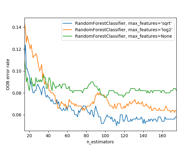
The sklearn docs show an example of the effects of different max_features choices, with increasing numbers of trees. In the plot, the blue plot line uses the fewest features and the green line uses the most (it uses all the features). As you can see in <<max_features>>, the models with the lowest error result from using a subset of features but with a larger number of trees.
随机森林的一个最重要的属性是,它们对超参数的选择不是很敏感,比如max_features。您可以将n_estimators设置为您有时间训练的尽可能高的数字—您拥有的树越多,模型就越准确。Max_samples通常可以保持默认值,除非您有超过20万个数据点,在这种情况下,将其设置为20万个将使它训练得更快,对精度的影响很小。Max_features =0.5和min_samples_leaf=4都可以很好地工作,尽管sklearn的默认值也可以很好地工作。
sklearn文档展示了一个不同max_features选项的效果示例,其中树的数量不断增加。在图中,蓝色的绘图线使用最少的特征,而绿色的线使用最多的特征(它使用了所有的特征)。正如您在<<max_features>>中所看到的,具有最低误差的模型来自使用特征子集但具有大量树。
To see the impact of n_estimators, let's get the predictions from each individual tree in our forest (these are in the estimators_ attribute):
为了查看n_estimators的影响,让我们获取森林中每棵树的预测结果(这些在estimators_属性中):
preds = np.stack([t.predict(valid_xs) for t in m.estimators_])As you can see, preds.mean(0) gives the same results as our random forest:
如你所见,preds.mean(0)给出了与我们的随机森林相同的结果:
r_mse(preds.mean(0), valid_y)Output
0.233975
Let's see what happens to the RMSE as we add more and more trees. As you can see, the improvement levels off quite a bit after around 30 trees:
让我们看看随着树的增加RMSE会发生什么变化。正如你所看到的,在大约 30 棵树之后,改进趋于平稳:
plt.plot([r_mse(preds[:i+1].mean(0), valid_y) for i in range(40)]);Output
<Figure size 432x288 with 1 Axes>

The performance on our validation set is worse than on our training set. But is that because we're overfitting, or because the validation set covers a different time period, or a bit of both? With the existing information we've seen, we can't tell. However, random forests have a very clever trick called out-of-bag (OOB) error that can help us with this (and more!).
在验证集上的性能比在训练集上的性能差。但这是因为我们过度拟合,还是因为验证集覆盖了不同的时间段,还是两者兼而有之?根据我们所看到的现有信息,我们无法判断。然而,随机森林有一个非常聪明的技巧,称为out-of-bag (OOB)误差,可以帮助我们解决这个问题(以及更多!)
Out-of-Bag Error
包外误差
Recall that in a random forest, each tree is trained on a different subset of the training data. The OOB error is a way of measuring prediction error on the training set by only including in the calculation of a row's error trees where that row was not included in training. This allows us to see whether the model is overfitting, without needing a separate validation set.
A: My intuition for this is that, since every tree was trained with a different randomly selected subset of rows, out-of-bag error is a little like imagining that every tree therefore also has its own validation set. That validation set is simply the rows that were not selected for that tree's training.
This is particularly beneficial in cases where we have only a small amount of training data, as it allows us to see whether our model generalizes without removing items to create a validation set. The OOB predictions are available in the oob_prediction_ attribute. Note that we compare them to the training labels, since this is being calculated on trees using the training set.
回想一下,在随机森林中,每棵树都是在训练数据的不同子集上训练的。OOB误差是一种在训练集上测量预测误差的方法,只需将该行未包含在训练中的错误树计算中。这使我们能够看到模型是否过拟合,而不需要单独的验证集。
A:我对此的直觉是,由于每棵树都是用不同的随机选择的行子集训练的,包外误差有点像想象每棵树因此也有自己的验证集。该验证集只是没有为该树的训练选择的行。
这在只有少量训练数据的情况下特别有用,因为它允许我们查看我们的模型在不删除项来创建验证集的情况下是否泛化。OOB预测在oob_prediction_属性中可用。注意,我们将它们与训练标签进行比较,因为这是使用训练集在树上计算的。
r_mse(m.oob_prediction_, y)Output
0.210681
We can see that our OOB error is much lower than our validation set error. This means that something else is causing that error, in addition to normal generalization error. We'll discuss the reasons for this later in this chapter.
我们可以看到,我们的OOB误差远低于我们的验证集误差。这意味着,除了正常的泛化误差,还有其他原因导致了这个误差。我们将在本章后面讨论造成这种情况的原因。
This is one way to interpret our model's predictions—let's focus on more of those now.
这是解释我们模型预测的一种方式——现在让我们关注更多的预测。
Model Interpretation
模型解释
For tabular data, model interpretation is particularly important. For a given model, the things we are most likely to be interested in are:
- How confident are we in our predictions using a particular row of data?
- For predicting with a particular row of data, what were the most important factors, and how did they influence that prediction?
- Which columns are the strongest predictors, which can we ignore?
- Which columns are effectively redundant with each other, for purposes of prediction?
- How do predictions vary, as we vary these columns?
As we will see, random forests are particularly well suited to answering these questions. Let's start with the first one!
对于表格数据,模型解释尤为重要。对于给定的模型,我们最有可能感兴趣的是:
- 我们对使用特定数据行进行预测有多大信心?
- 对于特定数据行的预测,最重要的因素是什么,它们是如何影响预测的?
- 哪些列是最强的预测因素,哪些可以忽略?
- 出于预测的目的,哪些列实际上是相互冗余的?
- 当我们改变这些列时,预测是如何变化的?
正如我们将看到的,随机森林特别适合回答这些问题。让我们从第一个开始!
Tree Variance for Prediction Confidence
预测置信度的树方差
We saw how the model averages the individual tree's predictions to get an overall prediction—that is, an estimate of the value. But how can we know the confidence of the estimate? One simple way is to use the standard deviation of predictions across the trees, instead of just the mean. This tells us the relative confidence of predictions. In general, we would want to be more cautious of using the results for rows where trees give very different results (higher standard deviations), compared to cases where they are more consistent (lower standard deviations).
In the earlier section on creating a random forest, we saw how to get predictions over the validation set, using a Python list comprehension to do this for each tree in the forest:
我们看到了该模型如何对单个树的预测进行平均以获得整体预测——即对值的估计。但是我们如何知道这个估计的置信度呢?一种简单的方法是使用树之间预测的标准差,而不仅仅是平均值。这告诉我们预测的相对置信度。一般来说,我们希望更谨慎地将结果用于树给出非常不同结果(更高的标准差)的行,而不是它们更一致的情况(更低的标准差)。
在前面关于创建随机森林的部分中,我们看到了如何通过验证集获得预测,使用Python 列表推导式对森林中的每棵树执行此操作:
preds = np.stack([t.predict(valid_xs) for t in m.estimators_])preds.shapeOutput
(40, 7988)
Now we have a prediction for every tree and every auction (40 trees and 7,988 auctions) in the validation set.
Using this we can get the standard deviation of the predictions over all the trees, for each auction:
现在,我们对验证集中的每棵树和每次拍卖(40棵树和7,988次拍卖)都有一个预测。
使用它,我们可以获得每次拍卖的所有树的预测标准差:
preds_std = preds.std(0)Here are the standard deviations for the predictions for the first five auctions—that is, the first five rows of the validation set:
下面是前五次拍卖(即验证集的前五行)的预测标准差:
preds_std[:5]Output
array([0.25065395, 0.11043862, 0.08242067, 0.26988508, 0.15730173])
As you can see, the confidence in the predictions varies widely. For some auctions, there is a low standard deviation because the trees agree. For others it's higher, as the trees don't agree. This is information that would be useful in a production setting; for instance, if you were using this model to decide what items to bid on at auction, a low-confidence prediction might cause you to look more carefully at an item before you made a bid.
正如你所看到的,对预测的置信度差异很大。对于一些拍卖,由于树木一致,所以标准差较低。对于其他拍卖,由于树木不一致,所以它更高。这是在生产环境中非常有用的信息;例如,如果你使用这个模型来决定拍卖中竞拍的物品,低置信度的预测可能会导致你在出价前更仔细地查看物品。
Feature Importance
特征重要性
It's not normally enough just to know that a model can make accurate predictions—we also want to know how it's making predictions. feature importance gives us insight into this. We can get these directly from sklearn's random forest by looking in the feature_importances_ attribute. Here's a simple function we can use to pop them into a DataFrame and sort them:
通常,仅仅知道一个模型能够做出准确的预测是不够的——我们还想知道它是如何做出预测的。特征重要性让我们能够深入了解这一点。我们可以通过查看feature_importances_属性直接从sklearn的随机森林中获得这些。下面是一个简单的函数,我们可以使用它将它们放入DataFrame并对它们进行排序:
def rf_feat_importance(m, df):
    return pd.DataFrame({'cols':df.columns, 'imp':m.feature_importances_}
                       ).sort_values('imp', ascending=False)
The feature importances for our model show that the first few most important columns have much higher importance scores than the rest, with (not surprisingly) YearMade and ProductSize being at the top of the list:
我们模型的特征重要性表明,前几个最重要的列的重要性分数比其他列高得多,(毫不奇怪)YearMade和ProductSize位于列表的顶部:
fi = rf_feat_importance(m, xs)
fi[:10]
Output
                  cols       imp
59            YearMade  0.180070
7          ProductSize  0.113915
31      Coupler_System  0.104699
8   fiProductClassDesc  0.064118
33     Hydraulics_Flow  0.059110
56             ModelID  0.059087
51         saleElapsed  0.051231
4      fiSecondaryDesc  0.041778
32      Grouser_Tracks  0.037560
2          fiModelDesc  0.030933
| cols | imp | |
|---|---|---|
| 59 | YearMade | 0.180070 |
| 7 | ProductSize | 0.113915 |
| 31 | Coupler_System | 0.104699 |
| 8 | fiProductClassDesc | 0.064118 |
| 33 | Hydraulics_Flow | 0.059110 |
| 56 | ModelID | 0.059087 |
| 51 | saleElapsed | 0.051231 |
| 4 | fiSecondaryDesc | 0.041778 |
| 32 | Grouser_Tracks | 0.037560 |
| 2 | fiModelDesc | 0.030933 |
A plot of the feature importances shows the relative importances more clearly:
特征重要性图更清楚地显示了相对重要性:
def plot_fi(fi):
    return fi.plot('cols', 'imp', 'barh', figsize=(12,7), legend=False)

plot_fi(fi[:30]);
Output
<Figure size 864x504 with 1 Axes>

The way these importances are calculated is quite simple yet elegant. The feature importance algorithm loops through each tree, and then recursively explores each branch. At each branch, it looks to see what feature was used for that split, and how much the model improves as a result of that split. The improvement (weighted by the number of rows in that group) is added to the importance score for that feature. This is summed across all branches of all trees, and finally the scores are normalized such that they add to 1.
计算这些重要性的方法非常简单而优雅。特征重要性算法循环遍历每棵树,然后递归地探索每个分支。在每个分支中,它会查看用于该拆分的特征,以及拆分后模型改进了多少。改进(由该组中的行数加权)被添加到该特征的重要性分数中。这是对所有树的所有分支的求和,最后将分数归一化,使它们加为1。
Removing Low-Importance Variables
删除低重要性变量
It seems likely that we could use just a subset of the columns by removing the variables of low importance and still get good results. Let's try just keeping those with a feature importance greater than 0.005:
似乎我们可以通过删除低重要性的变量来仅使用列的子集,并且仍然可以获得良好的结果。让我们尝试只保留特征重要性大于0.005的那些变量:
to_keep = fi[fi.imp>0.005].cols
len(to_keep)
Output
21
We can retrain our model using just this subset of the columns:
我们可以只使用列的这个子集来重新训练我们的模型:
xs_imp = xs[to_keep]
valid_xs_imp = valid_xs[to_keep]m = rf(xs_imp, y)And here's the result:
结果如下:
m_rmse(m, xs_imp, y), m_rmse(m, valid_xs_imp, valid_y)Output
(0.181204, 0.230329)
Our accuracy is about the same, but we have far fewer columns to study:
我们的准确性大致相同,但我们要研究的列要少得多:
len(xs.columns), len(xs_imp.columns)Output
(66, 21)
We've found that generally the first step to improving a model is simplifying it—78 columns was too many for us to study them all in depth! Furthermore, in practice often a simpler, more interpretable model is easier to roll out and maintain.
This also makes our feature importance plot easier to interpret. Let's look at it again:
我们发现,通常来说,改进模型的第一步是简化模型——78列太多了,我们无法深入研究它们!此外,在实践中,通常更简单、更可解释的模型更容易推广和维护。
这也使我们的特性重要性图更容易解释。让我们再看一遍:
plot_fi(rf_feat_importance(m, xs_imp));Output
<Figure size 864x504 with 1 Axes>

One thing that makes this harder to interpret is that there seem to be some variables with very similar meanings: for example, ProductGroup and ProductGroupDesc. Let's try to remove any redundent features.
使这更难解释的一件事是,似乎有一些变量具有非常相似的含义:例如,ProductGroup和ProductGroupDesc。让我们尝试删除所有冗余特征。
Removing Redundant Features
删除冗余特征
Let's start with:
让我们开始:
cluster_columns(xs_imp)Output
<Figure size 720x432 with 1 Axes>

In this chart, the pairs of columns that are most similar are the ones that were merged together early, far from the "root" of the tree at the left. Unsurprisingly, the fields ProductGroup and ProductGroupDesc were merged quite early, as were saleYear and saleElapsed and fiModelDesc and fiBaseModel. These might be so closely correlated they are practically synonyms for each other.
note: Determining Similarity: The most similar pairs are found by calculating the rank correlation, which means that all the values are replaced with their rank (i.e., first, second, third, etc. within the column), and then the correlation is calculated. (Feel free to skip over this minor detail though, since it's not going to come up again in the book!)
Let's try removing some of these closely related features to see if the model can be simplified without impacting the accuracy. First, we create a function that quickly trains a random forest and returns the OOB score, by using a lower max_samples and higher min_samples_leaf. The OOB score is a number returned by sklearn that ranges between 1.0 for a perfect model and 0.0 for a random model. (In statistics it's called R^2, although the details aren't important for this explanation.) We don't need it to be very accurate—we're just going to use it to compare different models, based on removing some of the possibly redundant columns:
在这个图表中,最相似的列对是早期合并在一起的列,远离左侧树的“根”。不出所料,字段ProductGroup和ProductGroupDesc很早就被合并了,就像saleYear和saleElapsed以及fiModelDesc和fiBaseModel一样。这些可能密切相关,实际上是彼此的同义词。
注意:确定相似度:通过计算 秩相关 找到最相似的对,这意味着所有值都被替换为它们的秩(即列中的第一、第二、第三等),然后计算相关性。(不过,请随意跳过这个小细节,因为它不会在书中再次出现!)
让我们尝试删除其中一些密切相关的特征,看看是否可以在不影响精度的情况下简化模型。首先,我们创建一个函数,通过使用较低的max_samples和较高的min_samples_leaf来快速训练一个随机森林并返回OOB分数。OOB分数是sklearn返回的一个数字,在1.0(完美模型)和0.0(随机模型)之间。(在统计学上,它被称为R^2,尽管细节对这个解释并不重要。)我们不需要它非常精确——我们只是要使用它来比较不同的模型,基于删除一些可能冗余的列:
def get_oob(df):
    m = RandomForestRegressor(n_estimators=40, min_samples_leaf=15,
        max_samples=50000, max_features=0.5, n_jobs=-1, oob_score=True)
    m.fit(df, y)
    return m.oob_score_
Here's our baseline:
这是我们的基线:
get_oob(xs_imp)Output
0.8768243241012634
Now we try removing each of our potentially redundant variables, one at a time:
现在,我们尝试一次删除一个潜在的冗余变量:
{c:get_oob(xs_imp.drop(c, axis=1)) for c in (
    'saleYear', 'saleElapsed', 'ProductGroupDesc','ProductGroup',
    'fiModelDesc', 'fiBaseModel',
    'Hydraulics_Flow','Grouser_Tracks', 'Coupler_System')}
Output
{'saleYear': 0.8766429216799364,
 'saleElapsed': 0.8725120463477113,
 'ProductGroupDesc': 0.8773289113713139,
 'ProductGroup': 0.8768277447901079,
 'fiModelDesc': 0.8760365396140016,
 'fiBaseModel': 0.8769194097714894,
 'Hydraulics_Flow': 0.8775975083138958,
 'Grouser_Tracks': 0.8780246481379101,
 'Coupler_System': 0.8780158691125818}
Now let's try dropping multiple variables. We'll drop one from each of the tightly aligned pairs we noticed earlier. Let's see what that does:
现在,让我们尝试删除多个变量。我们将从之前注意到的每个紧密对齐的对中删除一个。让我们看看它做了什么:
to_drop = ['saleYear', 'ProductGroupDesc', 'fiBaseModel', 'Grouser_Tracks']
get_oob(xs_imp.drop(to_drop, axis=1))
Output
0.8747772191306009
Looking good! This is really not much worse than the model with all the fields. Let's create DataFrames without these columns, and save them:
看上去不错!这真的不比包含所有字段的模型差多少。让我们创建没有这些列的DataFrames,并保存它们:
xs_final = xs_imp.drop(to_drop, axis=1)
valid_xs_final = valid_xs_imp.drop(to_drop, axis=1)save_pickle(path/'xs_final.pkl', xs_final)
save_pickle(path/'valid_xs_final.pkl', valid_xs_final)We can load them back later with:
我们可以稍后加载它们:
xs_final = load_pickle(path/'xs_final.pkl')
valid_xs_final = load_pickle(path/'valid_xs_final.pkl')
Now we can check our RMSE again, to confirm that the accuracy hasn't substantially changed.
现在我们可以再次检查我们的RMSE,以确认准确性没有实质性的改变。
m = rf(xs_final, y)
m_rmse(m, xs_final, y), m_rmse(m, valid_xs_final, valid_y)
Output
(0.183426, 0.231894)
By focusing on the most important variables, and removing some redundant ones, we've greatly simplified our model. Now, let's see how those variables affect our predictions using partial dependence plots.
通过关注最重要的变量并删除一些冗余的变量,我们大大简化了我们的模型。现在,让我们看看这些变量如何使用部分依赖图影响我们的预测。
Partial Dependence
部分依赖
As we've seen, the two most important predictors are ProductSize and YearMade. We'd like to understand the relationship between these predictors and sale price. It's a good idea to first check the count of values per category (provided by the Pandas value_counts method), to see how common each category is:
正如我们所看到的,两个最重要的预测因素是ProductSize和YearMade。我们想要了解这些预测因素与销售价格之间的关系。最好先检查每个类别的值的计数(由Pandas的value_counts方法提供),以了解每个类别的常见程度:
p = valid_xs_final['ProductSize'].value_counts(sort=False).plot.barh()
c = to.classes['ProductSize']
plt.yticks(range(len(c)), c);
Output
<Figure size 432x288 with 1 Axes>

The largrest group is #na#, which is the label fastai applies to missing values.
Let's do the same thing for YearMade. Since this is a numeric feature, we'll need to draw a histogram, which groups the year values into a few discrete bins:
最大的组是#na#,这是fastai标签应用于缺失值。
让我们为YearMade做同样的事情。由于这是一个数字特性,我们需要绘制一个直方图,将年份值分组到几个离散的 bin 中:
ax = valid_xs_final['YearMade'].hist()Output
<Figure size 432x288 with 1 Axes>

Other than the special value 1950 which we used for coding missing year values, most of the data is from after 1990.
Now we're ready to look at partial dependence plots. Partial dependence plots try to answer the question: if a row varied on nothing other than the feature in question, how would it impact the dependent variable?
For instance, how does YearMade impact sale price, all other things being equal?
To answer this question, we can't just take the average sale price for each YearMade. The problem with that approach is that many other things vary from year to year as well, such as which products are sold, how many products have air-conditioning, inflation, and so forth. So, merely averaging over all the auctions that have the same YearMade would also capture the effect of how every other field also changed along with YearMade and how that overall change affected price.
Instead, what we do is replace every single value in the YearMade column with 1950, and then calculate the predicted sale price for every auction, and take the average over all auctions. Then we do the same for 1951, 1952, and so forth until our final year of 2011. This isolates the effect of only YearMade (even if it does so by averaging over some imagined records where we assign a YearMade value that might never actually exist alongside some other values).
A: If you are philosophically minded it is somewhat dizzying to contemplate the different kinds of hypotheticality that we are juggling to make this calculation. First, there's the fact that every prediction is hypothetical, because we are not noting empirical data. Second, there's the point that we're not merely interested in asking how sale price would change if we changed
YearMadeand everything else along with it. Rather, we're very specifically asking, how sale price would change in a hypothetical world where onlyYearMadechanged. Phew! It is impressive that we can ask such questions. I recommend Judea Pearl and Dana Mackenzie's recent book on causality, The Book of Why (Basic Books), if you're interested in more deeply exploring formalisms for analyzing these subtleties.
With these averages, we can then plot each of these years on the x-axis, and each of the predictions on the y-axis. This, finally, is a partial dependence plot. Let's take a look:
除了我们用于编码缺失年份值的特殊值1950外,大多数数据来自1990年以后。
现在我们来看看部分依赖图。部分依赖图试图回答这个问题:如果一行只根据所讨论的特征而变化,它会如何影响因变量?
例如,在其他条件相同的情况下,YearMade如何影响销售价格?
要回答这个问题,我们不能只看YearMade的平均销售价格。这种方法的问题是,许多其他因素也因年而异,如销售哪些产品,有多少产品有空调,通货膨胀,等等。因此,仅仅对所有具有相同YearMade的拍卖进行平均,也可以捕捉到其他领域随着YearMade的变化的影响,以及整体变化如何影响价格。
相反,我们所做的是用1950代替YearMade列中的每个值,然后计算每次拍卖的预测销售价格,并取所有拍卖的平均值。然后我们对1951、1952等做同样的事情,直到最后一年2011。这隔离了仅YearMade的影响(即使它是通过对一些想象的记录进行平均来实现的,其中我们分配了一个YearMade值,这个值可能永远不会与其他值一起存在)。
A:如果你有哲学头脑,思考我们在做这个计算时要用到的不同种类的假设会令人眼花缭乱。首先, 每个 预测都是假设的,因为我们没有注意到经验数据。其次,我们不仅仅想知道如果我们改变
YearMade以及随之而来的其他一切,销售价格会发生怎样的变化。相反,我们非常具体地问,在一个只有YearMade改变的假设世界中,销售价格会如何变化。唷!令人印象深刻的是,我们可以提出这样的问题。如果你有兴趣更深入地探索分析这些微妙之处的形式主义,我推荐Judea Pearl 和Dana Mackenzie关于因果关系的新书《为什么之书》(基础书籍)。
有了这些平均值,我们可以在x轴上绘制这些年的每一年,在y轴上绘制每一个预测。最后,这是一个部分依赖图。让我们看一下:
from sklearn.inspection import plot_partial_dependence

fig,ax = plt.subplots(figsize=(12, 4))
plot_partial_dependence(m, valid_xs_final, ['YearMade','ProductSize'],
                        grid_resolution=20, ax=ax);
Output
<Figure size 864x288 with 3 Axes>

Looking first of all at the YearMade plot, and specifically at the section covering the years after 1990 (since as we noted this is where we have the most data), we can see a nearly linear relationship between year and price. Remember that our dependent variable is after taking the logarithm, so this means that in practice there is an exponential increase in price. This is what we would expect: depreciation is generally recognized as being a multiplicative factor over time, so, for a given sale date, varying year made ought to show an exponential relationship with sale price.
The ProductSize partial plot is a bit concerning. It shows that the final group, which we saw is for missing values, has the lowest price. To use this insight in practice, we would want to find out why it's missing so often, and what that means. Missing values can sometimes be useful predictors—it entirely depends on what causes them to be missing. Sometimes, however, they can indicate data leakage.
首先来看YearMade图,特别是涵盖1990年之后的部分(因为我们注意到这是我们拥有最多数据的部分),我们可以看到年份和价格之间几乎呈线性关系。请记住,我们的因变量是取对数后的,因为这意味着实际上价格呈指数增长。这就是我们所期望的:折旧通常被认为是随时间推移的乘法因素,因此,对于给定的销售日期,不同的年份应该与销售价格呈指数关系。
ProductSize部分图有点令人担忧。它表明,我们看到的最后一组是缺失值,价格最低。为了在实践中使用这种洞察力,我们想要找出为什么它经常缺失,以及这意味着什么。缺失值有时可能是有用的预测指标——这完全取决于导致它们缺失的原因。然而,有时它们可能表明数据泄漏。
Data Leakage
数据泄漏
In the paper "Leakage in Data Mining: Formulation, Detection, and Avoidance", Shachar Kaufman, Saharon Rosset, and Claudia Perlich describe leakage as:
: The introduction of information about the target of a data mining problem, which should not be legitimately available to mine from. A trivial example of leakage would be a model that uses the target itself as an input, thus concluding for example that 'it rains on rainy days'. In practice, the introduction of this illegitimate information is unintentional, and facilitated by the data collection, aggregation and preparation process.
They give as an example:
: A real-life business intelligence project at IBM where potential customers for certain products were identified, among other things, based on keywords found on their websites. This turned out to be leakage since the website content used for training had been sampled at the point in time where the potential customer has already become a customer, and where the website contained traces of the IBM products purchased, such as the word 'Websphere' (e.g., in a press release about the purchase or a specific product feature the client uses).
Data leakage is subtle and can take many forms. In particular, missing values often represent data leakage.
For instance, Jeremy competed in a Kaggle competition designed to predict which researchers would end up receiving research grants. The information was provided by a university and included thousands of examples of research projects, along with information about the researchers involved and data on whether or not each grant was eventually accepted. The university hoped to be able to use the models developed in this competition to rank which grant applications were most likely to succeed, so it could prioritize its processing.
Jeremy used a random forest to model the data, and then used feature importance to find out which features were most predictive. He noticed three surprising things:
- The model was able to correctly predict who would receive grants over 95% of the time.
- Apparently meaningless identifier columns were the most important predictors.
- The day of week and day of year columns were also highly predictive; for instance, the vast majority of grant applications dated on a Sunday were accepted, and many accepted grant applications were dated on January 1.
For the identifier columns, one partial dependence plot per column showed that when the information was missing the application was almost always rejected. It turned out that in practice, the university only filled out much of this information after a grant application was accepted. Often, for applications that were not accepted, it was just left blank. Therefore, this information was not something that was actually available at the time that the application was received, and it would not be available for a predictive model—it was data leakage.
In the same way, the final processing of successful applications was often done automatically as a batch at the end of the week, or the end of the year. It was this final processing date which ended up in the data, so again, this information, while predictive, was not actually available at the time that the application was received.
This example showcases the most practical and simple approaches to identifying data leakage, which are to build a model and then:
- Check whether the accuracy of the model is too good to be true.
- Look for important predictors that don't make sense in practice.
- Look for partial dependence plot results that don't make sense in practice.
Thinking back to our bear detector, this mirrors the advice that we provided in <<chapter_production>>—it is often a good idea to build a model first and then do your data cleaning, rather than vice versa. The model can help you identify potentially problematic data issues.
It can also help you identify which factors influence specific predictions, with tree interpreters.
在"数据挖掘中的泄漏:制定、检测和避免"一文中,Shachar Kaufman、Saharon Rosset和Claudia Perlich将泄漏描述为:
:引入关于数据挖掘问题目标的信息,这些信息不应合法地用于挖掘。泄漏的一个小例子是,一个模型将目标本身作为输入,从而得出“雨天下雨”的结论。在实践中,这种非法信息的引入是无意的,并通过数据收集、汇总和准备过程加以促进。
他们举了一个例子:
:IBM的一个真实商业智能项目,其中根据在其网站上找到的关键字确定了某些产品的潜在客户。这被证明是泄漏,因为用于训练的网站内容是在潜在客户已经成为客户的时间点进行采样的,并且该网站包含了购买的IBM产品的痕迹,例如“Websphere”一词(例如,在有关购买或客户使用的特定产品功能的新闻稿中)。
数据泄漏是微妙的,可以采取多种形式。特别是,缺失值通常表示数据泄漏。
例如,Jeremy参加了Kaggle竞赛,该竞赛旨在预测哪些研究人员最终会获得研究经费。这些信息是由一所大学提供的,其中包括数千个研究项目的例子,以及涉及的研究人员的信息,以及每项拨款申请是否最终被接受的数据。该大学希望能够使用在这次比赛中开发的模型来对最有可能成功拨款申请进行排名,以便优先处理。
Jeremy使用随机森林对数据进行建模,然后使用特征重要性来找出最具预测性的特征。他注意到三件令人惊讶的事情:
- 该模型能够在95%以上的情况下正确预测谁将获得拨款。
- 显然,无意义的标识符列是最重要的预测因素。
- 星期几和年月几列也具有高度的预测性;例如,绝大多数日期为周日的拨款申请被接受,许多被接受的拨款申请日期在1月1日。
对于标识符列,每列一个部分依赖图表明,当信息丢失时,申请几乎总是被拒绝。事实证明,在实践中,这所大学只是在拨款申请被接受后才填写了大部分信息。通常,对于那些没有被接受的申请,它只是留空。因此,在收到申请时,这些信息并不是实际可用的,也不适用于预测模型——这是数据泄漏。
同样,成功申请的最终处理通常是在周末或年底自动批量完成的。正是这个最终处理日期最终出现在数据中,所以,这些信息虽然具有预测性,但在收到申请时实际上是不可用的。
这个例子展示了识别数据泄漏的最实用和最简单的方法,即构建一个模型,然后:
- 检查模型的准确性是否好到不行。
- 寻找在实践中没有意义的重要预测因素。
- 寻找在实践中没有意义的部分依赖图结果。
回想一下我们的熊探测器,这反映了我们在<<chapter_production>>中提供的建议——首先构建一个模型然后进行数据清理通常是一个好主意,反之则不然。该模型可以帮助您识别潜在的问题数据问题。
它还可以通过树解释器帮助您确定哪些因素会影响特定的预测。
Tree Interpreter
树解释器
#hide
import warnings
warnings.simplefilter('ignore', FutureWarning)

from treeinterpreter import treeinterpreter
from waterfall_chart import plot as waterfall
At the start of this section, we said that we wanted to be able to answer five questions:
- How confident are we in our predictions using a particular row of data?
- For predicting with a particular row of data, what were the most important factors, and how did they influence that prediction?
- Which columns are the strongest predictors?
- Which columns are effectively redundant with each other, for purposes of prediction?
- How do predictions vary, as we vary these columns?
We've handled four of these already; only the second question remains. To answer this question, we need to use the treeinterpreter library. We'll also use the waterfallcharts library to draw the chart of the results.
!pip install treeinterpreter
!pip install waterfallcharts
在本节开始时,我们说过我们希望能够回答5个问题:
- 我们对使用特定数据行进行预测的信心有多大?
- 对于特定数据行的预测,最重要的因素是什么,它们是如何影响预测的?
- 哪些列是最强的预测因素?
- 出于预测的目的,哪些列实际上是相互冗余的?
- 当我们改变这些列时,预测是如何变化的?
我们已经处理了其中的四个;剩下的只有第二个问题了。要回答这个问题,我们需要使用treeinterpreter库。我们还将使用waterfallcharts库来绘制结果图表。
!pip install treeinterpreter
!pip install waterfallcharts
We have already seen how to compute feature importances across the entire random forest. The basic idea was to look at the contribution of each variable to improving the model, at each branch of every tree, and then add up all of these contributions per variable.
We can do exactly the same thing, but for just a single row of data. For instance, let's say we are looking at some particular item at auction. Our model might predict that this item will be very expensive, and we want to know why. So, we take that one row of data and put it through the first decision tree, looking to see what split is used at each point throughout the tree. For each split, we see what the increase or decrease in the addition is, compared to the parent node of the tree. We do this for every tree, and add up the total change in importance by split variable.
For instance, let's pick the first few rows of our validation set:
我们已经看到了如何计算整个随机森林的特征重要性。基本思想是在每棵树的每个分支上查看每个变量对改进模型的贡献,然后把每个变量的所有贡献相加。
我们可以做完全相同的事情,但是只针对一行数据。例如,假设我们正在拍卖某些特定的物品。我们的模型可能会预测这个物品会非常昂贵,我们想知道为什么。因此,我们将那一行数据放入第一棵决策树中,看看在树的每个点使用了什么拆分。对于每个拆分,我们可以看到与树的父节点相比,加法的增加或减少是什么。我们对每棵树都这样做,并通过拆分变量将重要性的总变化相加。
例如,让我们选择验证集的前几行
row = valid_xs_final.iloc[:5]We can then pass these to treeinterpreter:
然后我们可以将它们传递给treeinterpreter:
prediction,bias,contributions = treeinterpreter.predict(m, row.values)prediction is simply the prediction that the random forest makes. bias is the prediction based on taking the mean of the dependent variable (i.e., the model that is the root of every tree). contributions is the most interesting bit—it tells us the total change in predicition due to each of the independent variables. Therefore, the sum of contributions plus bias must equal the prediction, for each row. Let's look just at the first row:
prediction只是随机森林做出的预测。bias是基于对因变量(即作为每棵树根的模型)取平均值的预测。contributions是最有趣的一点——它告诉我们由于每个自变量而导致的预测的总变化。因此,每一行的contributions加bias之和必须等于prediction。让我们看看第一行:
prediction[0], bias[0], contributions[0].sum()Output
(array([10.01216396]), 10.104746057831765, -0.0925820990266335)
The clearest way to display the contributions is with a waterfall plot. This shows how the positive and negative contributions from all the independent variables sum up to create the final prediction, which is the righthand column labeled "net" here:
最清晰的显示贡献的方法是使用瀑布图。这显示了所有自变量的正负贡献是如何相加以创建最终预测的,即此处标记为“net”的右侧列:
waterfall(valid_xs_final.columns, contributions[0], threshold=0.08,
          rotation_value=45,formatting='{:,.3f}');
Output
<Figure size 432x288 with 1 Axes>

This kind of information is most useful in production, rather than during model development. You can use it to provide useful information to users of your data product about the underlying reasoning behind the predictions.
这种信息在生产中最有用,而不是在模型开发期间。您可以使用它向数据产品的用户提供有关预测背后的潜在推理的有用信息。
Now that we covered some classic machine learning techniques to solve this problem, let's see how deep learning can help!
现在,我们已经介绍了一些经典的机器学习技术来解决这个问题,让我们看看深度学习如何提供帮助!
Extrapolation and Neural Networks
外推和神经网络
A problem with random forests, like all machine learning or deep learning algorithms, is that they don't always generalize well to new data. We will see in which situations neural networks generalize better, but first, let's look at the extrapolation problem that random forests have.
与所有机器学习或深度学习算法一样,随机森林的一个问题是,它们并不总是能很好地泛化到新数据。我们将会看到神经网络在哪些情况下可以更好地泛化,但首先,让我们看看随机森林的外推问题。
The Extrapolation Problem
外推问题
#hide
np.random.seed(42)
Let's consider the simple task of making predictions from 40 data points showing a slightly noisy linear relationship:
让我们考虑从40个数据点进行预测的简单任务,这些数据点显示出略微有噪声的线性关系:
x_lin = torch.linspace(0,20, steps=40)
y_lin = x_lin + torch.randn_like(x_lin)
plt.scatter(x_lin, y_lin);
Output
<Figure size 432x288 with 1 Axes>

Although we only have a single independent variable, sklearn expects a matrix of independent variables, not a single vector. So we have to turn our vector into a matrix with one column. In other words, we have to change the shape from [40] to [40,1]. One way to do that is with the unsqueeze method, which adds a new unit axis to a tensor at the requested dimension:
虽然我们只有一个自变量,但是sklearn需要一个自变量矩阵,而不是一个向量。所以我们必须把我们的向量变成一个只有一列的矩阵。换句话说,我们必须将形状从[40]更改为[40,1]。一种方法是使用unsqueeze方法,它在被请求的维度上为张量添加一个新的单位轴:
xs_lin = x_lin.unsqueeze(1)
x_lin.shape,xs_lin.shape
Output
(torch.Size([40]), torch.Size([40, 1]))
A more flexible approach is to slice an array or tensor with the special value None, which introduces an additional unit axis at that location:
一种更灵活的方法是使用特殊值None对数组或张量进行切片,这会在该位置引入了一个额外的单位轴:
x_lin[:,None].shapeOutput
torch.Size([40, 1])
We can now create a random forest for this data. We'll use only the first 30 rows to train the model:
现在,我们可以为这些数据创建一个随机森林。我们将只使用前30行来训练模型:
m_lin = RandomForestRegressor().fit(xs_lin[:30],y_lin[:30])Then we'll test the model on the full dataset. The blue dots are the training data, and the red dots are the predictions:
然后,我们将在完整数据集上测试该模型。蓝点是训练数据,红点是预测:
plt.scatter(x_lin, y_lin, 20)
plt.scatter(x_lin, m_lin.predict(xs_lin), color='red', alpha=0.5);
Output
<Figure size 432x288 with 1 Axes>

We have a big problem! Our predictions outside of the domain that our training data covered are all too low. Why do you suppose this is?
Remember, a random forest just averages the predictions of a number of trees. And a tree simply predicts the average value of the rows in a leaf. Therefore, a tree and a random forest can never predict values outside of the range of the training data. This is particularly problematic for data where there is a trend over time, such as inflation, and you wish to make predictions for a future time. Your predictions will be systematically too low.
But the problem extends beyond time variables. Random forests are not able to extrapolate outside of the types of data they have seen, in a more general sense. That's why we need to make sure our validation set does not contain out-of-domain data.
我们有一个大问题!我们在训练数据涵盖的领域之外的预测都太低了。你认为这是为什么?
记住,随机森林只是对许多树的预测进行平均。一棵树只是预测叶子中行的平均值。因此,树和随机森林永远无法预测训练数据范围之外的值。这对于随着时间的推移存在趋势的数据(例如通货膨胀,并且您希望对未来时间进行预测)尤其成问题。你的预测会系统性地过低。
但是这个问题超越了时间变量。从更普遍的意义上说,随机森林无法推断他们所看到的数据类型之外的数据。这就是为什么我们需要确保验证集不包含域外数据。
Finding Out-of-Domain Data
查找域外数据
Sometimes it is hard to know whether your test set is distributed in the same way as your training data, or, if it is different, what columns reflect that difference. There's actually an easy way to figure this out, which is to use a random forest!
But in this case we don't use the random forest to predict our actual dependent variable. Instead, we try to predict whether a row is in the validation set or the training set. To see this in action, let's combine our training and validation sets together, create a dependent variable that represents which dataset each row comes from, build a random forest using that data, and get its feature importance:
有时很难知道测试集是否以与训练数据相同的方式分布,或者,如果不同,哪些列反映了这种差异。实际上有一个简单的方法可以解决这个问题,那就是使用随机森林!
但在这种情况下,我们不使用随机森林来预测我们实际的因变量。相反,我们试图预测一行是在验证集中还是在训练集中。要了解这一点,让我们将训练集和验证集结合在一起,创建一个因变量来表示每一行来自哪个数据集,使用该数据构建一个随机森林,并获得其特征重要性:
df_dom = pd.concat([xs_final, valid_xs_final])
is_valid = np.array([0]*len(xs_final) + [1]*len(valid_xs_final))

m = rf(df_dom, is_valid)
rf_feat_importance(m, df_dom)[:6]
Output
           cols       imp
6   saleElapsed  0.891571
9       SalesID  0.091174
14    MachineID  0.012950
0      YearMade  0.001520
10    Enclosure  0.000430
5       ModelID  0.000395
| cols | imp | |
|---|---|---|
| 6 | saleElapsed | 0.891571 |
| 9 | SalesID | 0.091174 |
| 14 | MachineID | 0.012950 |
| 0 | YearMade | 0.001520 |
| 10 | Enclosure | 0.000430 |
| 5 | ModelID | 0.000395 |
This shows that there are three columns that differ significantly between the training and validation sets: saleElapsed, SalesID, and MachineID. It's fairly obvious why this is the case for saleElapsed: it's the number of days between the start of the dataset and each row, so it directly encodes the date. The difference in SalesID suggests that identifiers for auction sales might increment over time. MachineID suggests something similar might be happening for individual items sold in those auctions.
Let's get a baseline of the original random forest model's RMSE, then see what the effect is of removing each of these columns in turn:
这表明训练集和验证集之间有三个明显不同的列:saleElapsed、SalesID和MachineID。对于saleElapsed来说,出现这种情况的原因非常明显:它是数据集开始到每行之间的天数,所以它直接对日期进行编码。SalesID的差异表明,拍卖销售的标识符可能会随着时间的推移而增加。MachineID表明在这些拍卖中出售的单个物品可能会发生类似的情况。
让我们获得原始随机森林模型的RMSE基线,然后看看依次删除这些列会产生什么影响:
m = rf(xs_final, y)
print('orig', m_rmse(m, valid_xs_final, valid_y))

for c in ('SalesID','saleElapsed','MachineID'):
    m = rf(xs_final.drop(c,axis=1), y)
    print(c, m_rmse(m, valid_xs_final.drop(c,axis=1), valid_y))
Output
orig 0.232883
SalesID 0.230347
saleElapsed 0.235529
MachineID 0.230735
It looks like we should be able to remove SalesID and MachineID without losing any accuracy. Let's check:
看起来我们应该能够删除SalesID和MachineID,而不会失去任何准确性。让我们检查:
time_vars = ['SalesID','MachineID']
xs_final_time = xs_final.drop(time_vars, axis=1)
valid_xs_time = valid_xs_final.drop(time_vars, axis=1)

m = rf(xs_final_time, y)
m_rmse(m, valid_xs_time, valid_y)
Output
0.229498
Removing these variables has slightly improved the model's accuracy; but more importantly, it should make it more resilient over time, and easier to maintain and understand. We recommend that for all datasets you try building a model where your dependent variable is is_valid, like we did here. It can often uncover subtle domain shift issues that you may otherwise miss.
One thing that might help in our case is to simply avoid using old data. Often, old data shows relationships that just aren't valid any more. Let's try just using the most recent few years of the data:
去除这些变量略微提高了模型的准确性;但更重要的是,随着时间的推移,它应该会使其更具弹性,更容易维护和理解。我们建议,您尝试为所有数据集构建一个因变量为is_valid的模型,就像我们在这里做的那样。它通常可以发现您可能会错过的微妙的域转移问题。
在我们的例子中,有一件事可能会有所帮助,那就是简单地避免使用旧数据。通常,旧数据显示不再有效的关系。让我们试着使用最近几年的数据:
xs['saleYear'].hist();Output
<Figure size 432x288 with 1 Axes>

Here's the result of training on this subset:
这是在这个子集上训练的结果:
filt = xs['saleYear']>2004
xs_filt = xs_final_time[filt]
y_filt = y[filt]m = rf(xs_filt, y_filt)
m_rmse(m, xs_filt, y_filt), m_rmse(m, valid_xs_time, valid_y)Output
(0.177284, 0.228008)
It's a tiny bit better, which shows that you shouldn't always just use your entire dataset; sometimes a subset can be better.
Let's see if using a neural network helps.
它稍微好一点,这表明你不应该总是只使用整个数据集;有时候子集可能会更好。
让我们看看使用神经网络是否有帮助。
Using a Neural Network
使用神经网络
We can use the same approach to build a neural network model. Let's first replicate the steps we took to set up the TabularPandas object:
我们可以用同样的方法来建立一个神经网络模型。让我们首先复制我们设置TabularPandas对象的步骤:
df_nn = pd.read_csv(path/'TrainAndValid.csv', low_memory=False)
df_nn['ProductSize'] = df_nn['ProductSize'].astype('category')
df_nn['ProductSize'].cat.set_categories(sizes, ordered=True, inplace=True)
df_nn[dep_var] = np.log(df_nn[dep_var])
df_nn = add_datepart(df_nn, 'saledate')
We can leverage the work we did to trim unwanted columns in the random forest by using the same set of columns for our neural network:
我们可以利用我们所做的工作,通过对我们的神经网络使用相同的列集来修剪随机森林中不需要的列:
df_nn_final = df_nn[list(xs_final_time.columns) + [dep_var]]Categorical columns are handled very differently in neural networks, compared to decision tree approaches. As we saw in <<chapter_collab>>, in a neural net a great way to handle categorical variables is by using embeddings. To create embeddings, fastai needs to determine which columns should be treated as categorical variables. It does this by comparing the number of distinct levels in the variable to the value of the max_card parameter. If it's lower, fastai will treat the variable as categorical. Embedding sizes larger than 10,000 should generally only be used after you've tested whether there are better ways to group the variable, so we'll use 9,000 as our max_card:
与决策树方法相比,神经网络中分类列的处理方式非常不同。正如我们在<<chapter_collab>>中看到的,在神经网络中处理分类变量的一个很好的方法是使用嵌入。为了创建嵌入,fastai需要确定哪些列应该被视为分类变量。它通过将变量中不同级别的数量与max_card参数的值进行比较来实现这一点。如果它更低,fastai将把这个变量视为分类变量。嵌入大小大于10,000通常只能在您测试是否有更好的方法对变量进行分组后使用,因此我们将使用9,000作为max_card:
cont_nn,cat_nn = cont_cat_split(df_nn_final, max_card=9000, dep_var=dep_var)In this case, there's one variable that we absolutely do not want to treat as categorical: the saleElapsed variable. A categorical variable cannot, by definition, extrapolate outside the range of values that it has seen, but we want to be able to predict auction sale prices in the future. Let's verify that cont_cat_split did the correct thing.
在这种情况下,有一个变量我们绝对不想将其视为分类变量:saleElapsed变量。根据定义,一个分类变量不能推断出它所看到的值范围之外的值,但我们希望能够预测未来的拍卖价格。让我们验证cont_cat_split是否做了正确的事情。
cont_nnOutput
['saleElapsed']
Let's take a look at the cardinality of each of the categorical variables that we have chosen so far:
让我们看看到目前为止我们选择的每个分类变量的基数:
df_nn_final[cat_nn].nunique()Output
YearMade                73
ProductSize              6
Coupler_System           2
fiProductClassDesc      74
Hydraulics_Flow          3
ModelID               5281
fiSecondaryDesc        177
fiModelDesc           5059
Enclosure                6
Hydraulics              12
ProductGroup             6
Drive_System             4
Tire_Size               17
dtype: int64
The fact that there are two variables pertaining to the "model" of the equipment, both with similar very high cardinalities, suggests that they may contain similar, redundant information. Note that we would not necessarily see this when analyzing redundant features, since that relies on similar variables being sorted in the same order (that is, they need to have similarly named levels). Having a column with 5,000 levels means needing 5,000 columns in our embedding matrix, which would be nice to avoid if possible. Let's see what the impact of removing one of these model columns has on the random forest:
有两个变量与设备的“模型”相关,它们都具有相似的非常高的基数,这一事实表明它们可能包含相似的冗余信息。请注意,在分析冗余特征时,我们不一定会看到这一点,因为这依赖于以相同顺序对相似变量进行排序(也就是说,它们需要具有相似的命名级别)。拥有5,000个级别的列意味着我们的嵌入矩阵中需要5,000列,如果可能的话,最好避免这种情况。让我们看看删除其中一个模型列对随机森林的影响:
xs_filt2 = xs_filt.drop('fiModelDescriptor', axis=1)
valid_xs_time2 = valid_xs_time.drop('fiModelDescriptor', axis=1)
m2 = rf(xs_filt2, y_filt)
m_rmse(m2, xs_filt2, y_filt), m_rmse(m2, valid_xs_time2, valid_y)
Output
(0.176713, 0.230195)
There's minimal impact, so we will remove it as a predictor for our neural network:
影响很小,所以我们将把它作为我们神经网络的预测器删除:
cat_nn.remove('fiModelDescriptor')We can create our TabularPandas object in the same way as when we created our random forest, with one very important addition: normalization. A random forest does not need any normalization—the tree building procedure cares only about the order of values in a variable, not at all about how they are scaled. But as we have seen, a neural network definitely does care about this. Therefore, we add the Normalize processor when we build our TabularPandas object:
我们可以像创建随机森林时一样创建我们的TablarPandas对象,其中有一个非常重要的补充:标准化。随机森林不需要任何规范化——树构建过程只关心变量中值的顺序,而不关心它们是如何缩放的。但正如我们所看到的,神经网络肯定会关心这一点。因此,当我们构建TabularPandas对象时,我们添加了Normalize处理器:
procs_nn = [Categorify, FillMissing, Normalize]
to_nn = TabularPandas(df_nn_final, procs_nn, cat_nn, cont_nn,
                      splits=splits, y_names=dep_var)
Tabular models and data don't generally require much GPU RAM, so we can use larger batch sizes:
表格模型和数据通常不需要太多GPU RAM,所以我们可以使用更大的批处理大小:
dls = to_nn.dataloaders(1024)As we've discussed, it's a good idea to set y_range for regression models, so let's find the min and max of our dependent variable:
正如我们所讨论的,为回归模型设置y_range是一个好主意,所以让我们找到因变量的最小和最大值:
y = to_nn.train.y
y.min(),y.max()
Output
(8.465899467468262, 11.863582611083984)
We can now create the Learner to create this tabular model. As usual, we use the application-specific learner function, to take advantage of its application-customized defaults. We set the loss function to MSE, since that's what this competition uses.
By default, for tabular data fastai creates a neural network with two hidden layers, with 200 and 100 activations, respectively. This works quite well for small datasets, but here we've got quite a large dataset, so we increase the layer sizes to 500 and 250:
我们现在可以创建Learner来创建这个表格模型。像往常一样,我们使用特定于应用程序的学习器函数,以利用其应用程序自定义的默认值。我们把损失函数设为MSE,因为这是本次比赛使用的。
默认情况下,对于表格数据,fastai会创建一个具有两个隐藏层的神经网络,分别具有200和100次激活。这对于小型数据集来说非常有效,但这里我们有一个相当大的数据集,所以我们将层大小增加到500和250:
learn = tabular_learner(dls, y_range=(8,12), layers=[500,250],
n_out=1, loss_func=F.mse_loss)learn.lr_find()Output
<IPython.core.display.HTML object>
SuggestedLRs(lr_min=0.002754228748381138, lr_steep=0.00015848931798245758)
<Figure size 432x288 with 1 Axes>

There's no need to use fine_tune, so we'll train with fit_one_cycle for a few epochs and see how it looks:
没有必要使用fine_tune,所以我们将使用fit_one_cycle进行几个epoch的训练,看看它怎么样:
learn.fit_one_cycle(5, 1e-2)Output
<IPython.core.display.HTML object>
| epoch | train_loss | valid_loss | time |
|---|---|---|---|
| 0 | 0.068459 | 0.061185 | 00:09 |
| 1 | 0.056469 | 0.058471 | 00:09 |
| 2 | 0.048689 | 0.052404 | 00:09 |
| 3 | 0.044529 | 0.052138 | 00:09 |
| 4 | 0.040860 | 0.051236 | 00:09 |
We can use our r_mse function to compare the result to the random forest result we got earlier:
我们可以使用我们的r_mse函数将结果与我们之前得到的随机森林结果进行比较:
preds,targs = learn.get_preds()
r_mse(preds,targs)
Output
<IPython.core.display.HTML object>
0.226353
It's quite a bit better than the random forest (although it took longer to train, and it's fussier about hyperparameter tuning).
Before we move on, let's save our model in case we want to come back to it again later:
它比随机森林要好得多(尽管它需要更长的训练时间,并且对超参数调优更麻烦)。
在我们继续之前,让我们保存我们的模型,以防我们以后想再次回到它:
learn.save('nn')Output
Path('models/nn.pth')Sidebar: fastai's Tabular Classes
侧边栏:fastai的表格类
In fastai, a tabular model is simply a model that takes columns of continuous or categorical data, and predicts a category (a classification model) or a continuous value (a regression model). Categorical independent variables are passed through an embedding, and concatenated, as we saw in the neural net we used for collaborative filtering, and then continuous variables are concatenated as well.
The model created in tabular_learner is an object of class TabularModel. Take a look at the source for tabular_learner now (remember, that's tabular_learner?? in Jupyter). You'll see that like collab_learner, it first calls get_emb_sz to calculate appropriate embedding sizes (you can override these by using the emb_szs parameter, which is a dictionary containing any column names you want to set sizes for manually), and it sets a few other defaults. Other than that, it just creates the TabularModel, and passes that to TabularLearner (note that TabularLearner is identical to Learner, except for a customized predict method).
That means that really all the work is happening in TabularModel, so take a look at the source for that now. With the exception of the BatchNorm1d and Dropout layers (which we'll be learning about shortly), you now have the knowledge required to understand this whole class. Take a look at the discussion of EmbeddingNN at the end of the last chapter. Recall that it passed n_cont=0 to TabularModel. We now can see why that was: because there are zero continuous variables (in fastai the n_ prefix means "number of," and cont is an abbreviation for "continuous").
在fastai中,表格模型是一个简单的模型,它采用连续或分类数据列,并预测类别(分类模型)或连续值(回归模型)。类别自变量通过嵌入并连接,就像我们在用于协同过滤的神经网络中看到的那样,然后连续变量也被连接起来。
在tabular_learner中创建的模型是TabularModel类的一个对象。现在看一下tabular_learner的源代码(记住,这是Jupyter中的tabular_learner??)。您将看到,与collab_learner一样,它首先调用get_emb_sz来计算适当的嵌入大小(您可以使用emb_szs参数来覆盖它们,它是一个字典,包含您想要手动设置大小的任何列名),它还设置了一些其他默认值。除此之外,它只是创建TabularModel,并将其传递给TabularLearner(请注意,除了定制的predict方法外,TabularLearner和Learner是相同的)。
这意味着实际上所有的工作都发生在TabularModel中,所以现在看看它的源代码。除了BatchNorm1d和Dropout层(我们将很快学习),您现在已经具备了理解整个类所需的知识。看看上一章末尾对EmbeddingNN的讨论。回想一下,它将n_cont=0传递给TabularModel。我们现在可以明白为什么会这样了:因为没有连续变量(在fastai中,n_前缀表示“数量”,而cont是“连续”的缩写)。
End sidebar
结束侧边栏
Another thing that can help with generalization is to use several models and average their predictions—a technique, as mentioned earlier, known as ensembling.
另一件有助于泛化的事情是使用多个模型并平均它们的预测——如前所述,这种技术称为集成。
Ensembling
集成
Think back to the original reasoning behind why random forests work so well: each tree has errors, but those errors are not correlated with each other, so the average of those errors should tend towards zero once there are enough trees. Similar reasoning could be used to consider averaging the predictions of models trained using different algorithms.
In our case, we have two very different models, trained using very different algorithms: a random forest, and a neural network. It would be reasonable to expect that the kinds of errors that each one makes would be quite different. Therefore, we might expect that the average of their predictions would be better than either one's individual predictions.
As we saw earlier, a random forest is itself an ensemble. But we can then include a random forest in another ensemble—an ensemble of the random forest and the neural network! While ensembling won't make the difference between a successful and an unsuccessful modeling process, it can certainly add a nice little boost to any models that you have built.
One minor issue we have to be aware of is that our PyTorch model and our sklearn model create data of different types: PyTorch gives us a rank-2 tensor (i.e, a column matrix), whereas NumPy gives us a rank-1 array (a vector). squeeze removes any unit axes from a tensor, and to_np converts it into a NumPy array:
回想一下为什么随机森林如此有效的最初原因:每棵树都有误差,但这些误差彼此之间并不相关,所以一旦有足够多的树,这些误差的平均值应该趋于零。类似的推理可以用来考虑平均使用不同算法训练的模型的预测。
在我们的例子中,我们有两个非常不同的模型,使用非常不同的算法训练:随机森林和神经网络。我们可以合理地预期,每个人犯的错误类型会非常不同。因此,我们可能期望他们预测的平均值会比任何一个人的预测要好。
正如我们之前看到的,随机森林本身就是一个集成。但是我们可以在另一个集成中包含一个随机森林——一个随机森林和神经网络的集成!虽然集成不会影响建模过程的成功与否,但它肯定可以为您所构建的任何模型增加一个不错的小改进。
我们必须注意的一个小问题是,PyTorch模型和sklearn模型创建了不同类型的数据:PyTorch给我们一个秩2张量(即列矩阵),而NumPy给我们一个秩1数组(一个向量).squeeze从一个张量中删除任何单位轴,to_np将其转换为NumPy数组:
rf_preds = m.predict(valid_xs_time)
ens_preds = (to_np(preds.squeeze()) + rf_preds) /2
This gives us a better result than either model achieved on its own:
这为我们提供了比单独实现的任何一种模型更好的结果:
r_mse(ens_preds,valid_y)Output
0.222134
In fact, this result is better than any score shown on the Kaggle leaderboard. It's not directly comparable, however, because the Kaggle leaderboard uses a separate dataset that we do not have access to. Kaggle does not allow us to submit to this old competition to find out how we would have done, but our results certainly look very encouraging!
事实上,这个结果比Kaggle排行榜上显示的任何分数都要好。但这并不具有直接可比性,因为Kaggle排行榜使用了我们无法访问的单独数据集。Kaggle不允许我们提交给这个旧的比赛来看看我们会怎么做,但是我们的结果看起来确实非常令人鼓舞!
Boosting
So far our approach to ensembling has been to use bagging, which involves combining many models (each trained on a different data subset) together by averaging them. As we saw, when this is applied to decision trees, this is called a random forest.
There is another important approach to ensembling, called boosting, where we add models instead of averaging them. Here is how boosting works:
- Train a small model that underfits your dataset.
- Calculate the predictions in the training set for this model.
- Subtract the predictions from the targets; these are called the "residuals" and represent the error for each point in the training set.
- Go back to step 1, but instead of using the original targets, use the residuals as the targets for the training.
- Continue doing this until you reach some stopping criterion, such as a maximum number of trees, or you observe your validation set error getting worse.
Using this approach, each new tree will be attempting to fit the error of all of the previous trees combined. Because we are continually creating new residuals, by subtracting the predictions of each new tree from the residuals from the previous tree, the residuals will get smaller and smaller.
To make predictions with an ensemble of boosted trees, we calculate the predictions from each tree, and then add them all together. There are many models following this basic approach, and many names for the same models. Gradient boosting machines (GBMs) and gradient boosted decision trees (GBDTs) are the terms you're most likely to come across, or you may see the names of specific libraries implementing these; at the time of writing, XGBoost is the most popular.
Note that, unlike with random forests, with this approach there is nothing to stop us from overfitting. Using more trees in a random forest does not lead to overfitting, because each tree is independent of the others. But in a boosted ensemble, the more trees you have, the better the training error becomes, and eventually you will see overfitting on the validation set.
We are not going to go into detail on how to train a gradient boosted tree ensemble here, because the field is moving rapidly, and any guidance we give will almost certainly be outdated by the time you read this. As we write this, sklearn has just added a HistGradientBoostingRegressor class that provides excellent performance. There are many hyperparameters to tweak for this class, and for all gradient boosted tree methods we have seen. Unlike random forests, gradient boosted trees are extremely sensitive to the choices of these hyperparameters; in practice, most people use a loop that tries a range of different hyperparameters to find the ones that work best.
到目前为止,我们的集成方法一直是使用bagging,它涉及到通过平均将许多模型(每个模型在不同的数据子集上训练)组合在一起。正如我们所看到的,当它应用于决策树时,它被称为随机森林。
还有另一种重要的集成方法,称为boosting,我们添加模型,而不是平均它们。以下是boosting的工作原理:
- 训练一个不适合您的数据集的小型模型。
- 计算该模型在训练集中的预测。
- 从目标中减去预测;这些被称为“残差”,代表训练集中每个点的误差。
- 回到第1步,但不是使用原始目标,而是使用残差作为训练目标。
- 继续这样做,直到达到某个停止条件,例如树的最大数目,或者观察到验证集错误变得更糟。
使用这种方法,每棵新树都将尝试拟合所有先前树组合的误差。因为我们不断地创造新的残差,通过从前一棵树的残差中减去每棵新树的预测,残差会越来越小。
为了使用增强树的集合进行预测,我们计算每棵树的预测,然后将它们加在一起。有许多模型遵循这种基本方法,并且对相同的模型有许多名称。梯度提升机(GBMs)和梯度提升决策树(GBDTs)是您最可能遇到的术语,或者您可能会看到实现这些的特定库的名称;在撰写本文时,XGBoost是最受欢迎的。
请注意,与随机森林不同,这种方法没有任何东西可以阻止我们过度拟合。在随机森林中使用更多的树不会导致过拟合,因为每棵树都是独立于其他树的。但在增强的集成中,树越多,训练误差就越低,最终你会在验证集上看到过拟合。
我们不会在这里详细介绍如何训练一个梯度增强树集成,因为这个领域正在快速发展,我们给出的任何指导几乎肯定会在你读到这篇文章的时候过时。在我们写这篇文章的时候,sklearn刚刚添加了一个HistGradientBoostingRegressor类,它提供了出色的性能。对于这个类,以及我们见过的所有梯度增强树方法,有许多超参数需要调整。与随机森林不同,梯度增强树对这些超参数的选择极其敏感;在实践中,大多数人使用循环来尝试一系列不同的超参数,以找到最有效的超参数。
One more technique that has gotten great results is to use embeddings learned by a neural net in a machine learning model.
另一项取得了巨大成果的技术是在机器学习模型中使用神经网络学习的嵌入。
Combining Embeddings with Other Methods
将嵌入与其他方法相结合
The abstract of the entity embedding paper we mentioned at the start of this chapter states: "the embeddings obtained from the trained neural network boost the performance of all tested machine learning methods considerably when used as the input features instead". It includes the very interesting table in <<embedding_mixed>>.
我们在本章开头提到的实体嵌入论文的摘要指出:“从训练过的神经网络获得的嵌入,在用作输入特征时,大大提高了所有测试机器学习方法的性能”。它包含了<<embedding_mixed>>中非常有趣的表格。
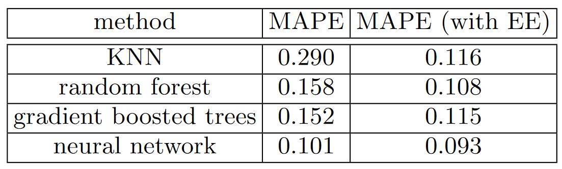
This is showing the mean average percent error (MAPE) compared among four different modeling techniques, three of which we have already seen, along with k-nearest neighbors (KNN), which is a very simple baseline method. The first numeric column contains the results of using the methods on the data provided in the competition; the second column shows what happens if you first train a neural network with categorical embeddings, and then use those categorical embeddings instead of the raw categorical columns in the model. As you see, in every case, the models are dramatically improved by using the embeddings instead of the raw categories.
This is a really important result, because it shows that you can get much of the performance improvement of a neural network without actually having to use a neural network at inference time. You could just use an embedding, which is literally just an array lookup, along with a small decision tree ensemble.
These embeddings need not even be necessarily learned separately for each model or task in an organization. Instead, once a set of embeddings are learned for some column for some task, they could be stored in a central place, and reused across multiple models. In fact, we know from private communication with other practitioners at large companies that this is already happening in many places.
这显示了四种不同建模技术之间的平均百分比误差(MAPE),其中三种我们已经见过,以及k近邻(KNN),这是一种非常简单的基线方法。第一个数字列包含对比赛中提供的数据使用方法的结果;第二列显示了如果您首先使用分类嵌入训练神经网络,然后使用这些分类嵌入而不是模型中原始的分类列会发生什么。正如您所看到的,在每种情况下,使用嵌入而不是原始类别都会显着改进模型。
这是一个非常重要的结果,因为它表明您可以获得神经网络的大部分性能改进,而无需在推理时实际使用神经网络。您可以只使用嵌入,它实际上只是一个数组查找,以及一个小型决策树集成。
这些嵌入甚至不需要为组织中的每个模型或任务单独学习。相反,一旦为某个任务的某个列学习了一组嵌入,它们就可以存储在一个中心位置,并在多个模型中重用。事实上,我们从与其他大公司从业者的私下交流中了解到,这已经在许多地方发生了。
Conclusion: Our Advice for Tabular Modeling
结论:我们对表格建模的建议
We have dicussed two approaches to tabular modeling: decision tree ensembles and neural networks. We've also mentioned two different decision tree ensembles: random forests, and gradient boosting machines. Each is very effective, but each also has compromises:
-
Random forests are the easiest to train, because they are extremely resilient to hyperparameter choices and require very little preprocessing. They are very fast to train, and should not overfit if you have enough trees. But they can be a little less accurate, especially if extrapolation is required, such as predicting future time periods.
-
Gradient boosting machines in theory are just as fast to train as random forests, but in practice you will have to try lots of different hyperparameters. They can overfit, but they are often a little more accurate than random forests.
-
Neural networks take the longest time to train, and require extra preprocessing, such as normalization; this normalization needs to be used at inference time as well. They can provide great results and extrapolate well, but only if you are careful with your hyperparameters and take care to avoid overfitting.
We suggest starting your analysis with a random forest. This will give you a strong baseline, and you can be confident that it's a reasonable starting point. You can then use that model for feature selection and partial dependence analysis, to get a better understanding of your data.
From that foundation, you can try neural nets and GBMs, and if they give you significantly better results on your validation set in a reasonable amount of time, you can use them. If decision tree ensembles are working well for you, try adding the embeddings for the categorical variables to the data, and see if that helps your decision trees learn better.
我们已经讨论了表格建模的两种方法:决策树集成和神经网络。我们还提到了两种不同的决策树集成:随机森林和梯度增强机。每种方法都非常有效,但也都有妥协:
-
随机森林是最容易训练的,因为它们对超参数选择具有极强的弹性,并且只需要很少的预处理。它们训练起来非常快,如果你有足够的树,就不会过拟合。但它们可能不太准确,尤其是在需要外推的情况下,比如预测未来的时间段。
-
理论上,梯度增强机的训练速度和随机森林一样快,但在实践中,你必须尝试许多不同的超参数。它们可能过度拟合,但它们通常比随机森林更准确一些。
-
神经网络的训练时间最长,需要额外的预处理,如归一化;这种归一化也需要在推理时使用。它们可以提供很好的结果和很好的推断,但前提是你要小心使用超参数,并注意避免过拟合。
我们建议从一个随机森林开始你的分析。这将为您提供强大的基线,并且您可以确信这是一个合理的起点。然后您可以使用该模型进行特征选择和部分依赖分析,以更好地理解您的数据。
在此基础上,您可以尝试神经网络和GBM,如果它们在合理的时间内为您的验证集提供了更好的结果,那么您可以使用它们。如果决策树集成对您来说效果很好,请尝试将分类变量的嵌入添加到数据中,看看这是否能帮助你的决策树更好地学习。
Questionnaire
问卷调查
- What is a continuous variable?
- What is a categorical variable?
- Provide two of the words that are used for the possible values of a categorical variable.
- What is a "dense layer"?
- How do entity embeddings reduce memory usage and speed up neural networks?
- What kinds of datasets are entity embeddings especially useful for?
- What are the two main families of machine learning algorithms?
- Why do some categorical columns need a special ordering in their classes? How do you do this in Pandas?
- Summarize what a decision tree algorithm does.
- Why is a date different from a regular categorical or continuous variable, and how can you preprocess it to allow it to be used in a model?
- Should you pick a random validation set in the bulldozer competition? If no, what kind of validation set should you pick?
- What is pickle and what is it useful for?
- How are
mse,samples, andvaluescalculated in the decision tree drawn in this chapter? - How do we deal with outliers, before building a decision tree?
- How do we handle categorical variables in a decision tree?
- What is bagging?
- What is the difference between
max_samplesandmax_featureswhen creating a random forest? - If you increase
n_estimatorsto a very high value, can that lead to overfitting? Why or why not? - In the section "Creating a Random Forest", just after <<max_features>>, why did
preds.mean(0)give the same result as our random forest? - What is "out-of-bag-error"?
- Make a list of reasons why a model's validation set error might be worse than the OOB error. How could you test your hypotheses?
- Explain why random forests are well suited to answering each of the following question:
- How confident are we in our predictions using a particular row of data?
- For predicting with a particular row of data, what were the most important factors, and how did they influence that prediction?
- Which columns are the strongest predictors?
- How do predictions vary as we vary these columns?
- What's the purpose of removing unimportant variables?
- What's a good type of plot for showing tree interpreter results?
- What is the "extrapolation problem"?
- How can you tell if your test or validation set is distributed in a different way than your training set?
- Why do we ensure
saleElapsedis a continuous variable, even although it has less than 9,000 distinct values? - What is "boosting"?
- How could we use embeddings with a random forest? Would we expect this to help?
- Why might we not always use a neural net for tabular modeling?
-
什么是连续变量?
-
什么是分类变量?
-
提供两个用于分类变量可能值的词。
-
什么是“致密层”?
-
实体嵌入如何减少内存使用并加速神经网络?
-
实体嵌入对哪些类型的数据集特别有用?
-
机器学习算法的两个主要家族是什么?
-
为什么某些分类列需要在其类中进行特殊排序?你是如何在Pandas中做到这一点的?
-
总结一下决策树算法的作用。
-
为什么日期不同于常规的分类变量或连续变量,如何对其进行预处理以使其在模型中使用?
-
您应该在推土机竞赛中选择一个随机的验证集吗?如果没有,应该选择什么样的验证集?
-
泡菜是什么,有什么用?
-
如何在本章绘制的决策树中计算
mse、samples和values? -
在构建决策树之前,我们如何处理异常值?
-
我们如何处理决策树中的分类变量?
-
什么是bagging?
-
创建随机森林时,
max_samples和max_features有什么区别? -
如果将
n_estimators增加到一个非常高的值,会导致过拟合吗?为什么或为什么不? -
在“创建随机森林”一节中,就在<<max_features>>之后,为什么
preds.mean(0)给出了与我们的随机森林相同的结果? -
“包外误差”是什么?
-
列出模型的验证集误差可能比OOB误差更严重的原因。你如何验证你的假设?
-
解释为什么随机森林很适合回答以下问题:
- 我们对使用特定数据行进行预测的信心有多大?
- 对于使用特定的数据行进行预测,最重要的因素是什么,它们是如何影响预测的?
- 哪些列是最强的预测因素?
- 当我们改变这些列时,预测如何变化?
-
删除不重要变量的目的是什么?
-
显示树解释器结果的最佳绘图类型是什么?
-
什么是“外推问题”?
-
您如何判断您的测试或验证集的分布方式是否与您的训练集不同?
-
为什么我们要确保
saleElapsed是一个连续变量,即使它的不同值少于9000个? -
什么是“boosting”?
-
我们如何在随机森林中使用嵌入?我们能指望这有帮助吗?
-
为什么我们不总是使用神经网络来进行表格建模?
Further Research
进一步的研究
- Pick a competition on Kaggle with tabular data (current or past) and try to adapt the techniques seen in this chapter to get the best possible results. Compare your results to the private leaderboard.
- Implement the decision tree algorithm in this chapter from scratch yourself, and try it on the dataset you used in the first exercise.
- Use the embeddings from the neural net in this chapter in a random forest, and see if you can improve on the random forest results we saw.
- Explain what each line of the source of
TabularModeldoes (with the exception of theBatchNorm1dandDropoutlayers).
- 在Kaggle上选择一个表格数据(当前或过去)的竞赛,并尝试采用本章中看到的技术来获得最佳结果。将你的结果与私人排行榜进行比较。
- 自己从头开始实现本章中的决策树算法,并在第一个练习中使用的数据集上进行尝试。
- 在随机森林中使用本章中神经网络的嵌入,看看你是否能改进我们看到的随机森林结果。
- 解释
TabularModel源码的每一行的作用(BatchNorm1d和Dropout层除外)。