%load_ext d2lbook.tab
tab.interact_select('mxnet', 'pytorch', 'tensorflow', 'jax')

Self-Attention and Positional Encoding

In deep learning, we often use CNNs or RNNs to encode sequences. Now with attention mechanisms in mind, imagine feeding a sequence of tokens into an attention mechanism such that at every step, each token has its own query, keys, and values. Here, when computing the value of a token's representation at the next layer, the token can attend (via its query vector) to any other's token (matching based on their key vectors). Using the full set of query-key compatibility scores, we can compute, for each token, a representation by building the appropriate weighted sum over the other tokens. Because every token is attending to each other token (unlike the case where decoder steps attend to encoder steps), such architectures are typically described as self-attention models Lin.Feng.Santos.ea.2017,Vaswani.Shazeer.Parmar.ea.2017, and elsewhere described as intra-attention model Cheng.Dong.Lapata.2016,Parikh.Tackstrom.Das.ea.2016,Paulus.Xiong.Socher.2017. In this section, we will discuss sequence encoding using self-attention, including using additional information for the sequence order.

%%tab mxnet
from d2l import mxnet as d2l
import math
from mxnet import autograd, np, npx
from mxnet.gluon import nn
npx.set_np()

%%tab pytorch
from d2l import torch as d2l
import math
import torch
from torch import nn

%%tab tensorflow
from d2l import tensorflow as d2l
import numpy as np
import tensorflow as tf

%%tab jax
from d2l import jax as d2l
from flax import linen as nn
from jax import numpy as jnp
import jax

[Self-Attention]

Given a sequence of input tokens $\mathbf{x}_1, \ldots, \mathbf{x}_n$ where any $\mathbf{x}_i \in \mathbb{R}^d$ ($1 \leq i \leq n$), its self-attention outputs a sequence of the same length $\mathbf{y}_1, \ldots, \mathbf{y}_n$, where

$\mathbf{y}_i = f(\mathbf{x}_i, (\mathbf{x}_1, \mathbf{x}_1), \ldots, (\mathbf{x}_n, \mathbf{x}_n)) \in \mathbb{R}^d$

according to the definition of attention pooling in eq_attention_pooling. Using multi-head attention, the following code snippet computes the self-attention of a tensor with shape (batch size, number of time steps or sequence length in tokens, $d$). The output tensor has the same shape.

%%tab pytorch
num_hiddens, num_heads = 100, 5
attention = d2l.MultiHeadAttention(num_hiddens, num_heads, 0.5)
batch_size, num_queries, valid_lens = 2, 4, d2l.tensor([3, 2])
X = d2l.ones((batch_size, num_queries, num_hiddens))
d2l.check_shape(attention(X, X, X, valid_lens),
                (batch_size, num_queries, num_hiddens))

%%tab mxnet
num_hiddens, num_heads = 100, 5
attention = d2l.MultiHeadAttention(num_hiddens, num_heads, 0.5)
attention.initialize()

%%tab jax
num_hiddens, num_heads = 100, 5
attention = d2l.MultiHeadAttention(num_hiddens, num_heads, 0.5)

%%tab tensorflow
num_hiddens, num_heads = 100, 5
attention = d2l.MultiHeadAttention(num_hiddens, num_hiddens, num_hiddens,
                                   num_hiddens, num_heads, 0.5)

%%tab mxnet
batch_size, num_queries, valid_lens = 2, 4, d2l.tensor([3, 2])
X = d2l.ones((batch_size, num_queries, num_hiddens))
d2l.check_shape(attention(X, X, X, valid_lens),
                (batch_size, num_queries, num_hiddens))

%%tab tensorflow
batch_size, num_queries, valid_lens = 2, 4, tf.constant([3, 2])
X = tf.ones((batch_size, num_queries, num_hiddens))
d2l.check_shape(attention(X, X, X, valid_lens, training=False),
                (batch_size, num_queries, num_hiddens))

%%tab jax
batch_size, num_queries, valid_lens = 2, 4, d2l.tensor([3, 2])
X = d2l.ones((batch_size, num_queries, num_hiddens))
d2l.check_shape(attention.init_with_output(d2l.get_key(), X, X, X, valid_lens,
                                           training=False)[0][0],
                (batch_size, num_queries, num_hiddens))

Comparing CNNs, RNNs, and Self-Attention

Let's compare architectures for mapping a sequence of $n$ tokens to another one of equal length, where each input or output token is represented by a $d$-dimensional vector. Specifically, we will consider CNNs, RNNs, and self-attention. We will compare their computational complexity, sequential operations, and maximum path lengths. Note that sequential operations prevent parallel computation, while a shorter path between any combination of sequence positions makes it easier to learn long-range dependencies within the sequence Hochreiter.Bengio.Frasconi.ea.2001.

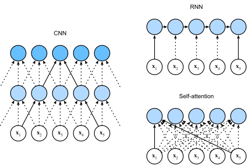
Let's regard any text sequence as a "one-dimensional image". Similarly, one-dimensional CNNs can process local features such as $n$-grams in text. Given a sequence of length $n$, consider a convolutional layer whose kernel size is $k$, and whose numbers of input and output channels are both $d$. The computational complexity of the convolutional layer is $\mathcal{O}(knd^2)$. As fig_cnn-rnn-self-attention shows, CNNs are hierarchical, so there are $\mathcal{O}(1)$ sequential operations and the maximum path length is $\mathcal{O}(n/k)$. For example, $\mathbf{x}_1$ and $\mathbf{x}_5$ are within the receptive field of a two-layer CNN with kernel size 3 in fig_cnn-rnn-self-attention.

When updating the hidden state of RNNs, multiplication of the $d \times d$ weight matrix and the $d$-dimensional hidden state has a computational complexity of $\mathcal{O}(d^2)$. Since the sequence length is $n$, the computational complexity of the recurrent layer is $\mathcal{O}(nd^2)$. According to fig_cnn-rnn-self-attention, there are $\mathcal{O}(n)$ sequential operations that cannot be parallelized and the maximum path length is also $\mathcal{O}(n)$.

In self-attention, the queries, keys, and values are all $n \times d$ matrices. Consider the scaled dot product attention in eq_softmax_QK_V, where an $n \times d$ matrix is multiplied by a $d \times n$ matrix, then the output $n \times n$ matrix is multiplied by an $n \times d$ matrix. As a result, the self-attention has a $\mathcal{O}(n^2d)$ computational complexity. As we can see from fig_cnn-rnn-self-attention, each token is directly connected to any other token via self-attention. Therefore, computation can be parallel with $\mathcal{O}(1)$ sequential operations and the maximum path length is also $\mathcal{O}(1)$.

All in all, both CNNs and self-attention enjoy parallel computation and self-attention has the shortest maximum path length. However, the quadratic computational complexity with respect to the sequence length makes self-attention prohibitively slow for very long sequences.

[Positional Encoding]

Unlike RNNs, which recurrently process tokens of a sequence one-by-one, self-attention ditches sequential operations in favor of parallel computation. Note that self-attention by itself does not preserve the order of the sequence. What do we do if it really matters that the model knows in which order the input sequence arrived?

The dominant approach for preserving information about the order of tokens is to represent this to the model as an additional input associated with each token. These inputs are called positional encodings, and they can either be learned or fixed a priori. We now describe a simple scheme for fixed positional encodings based on sine and cosine functions Vaswani.Shazeer.Parmar.ea.2017.

Suppose that the input representation $\mathbf{X} \in \mathbb{R}^{n \times d}$ contains the $d$-dimensional embeddings for $n$ tokens of a sequence. The positional encoding outputs $\mathbf{X} + \mathbf{P}$ using a positional embedding matrix $\mathbf{P} \in \mathbb{R}^{n \times d}$ of the same shape, whose element on the $i^\textrm{th}$ row and the $(2j)^\textrm{th}$ or the $(2j + 1)^\textrm{th}$ column is

$\begin{aligned} p_{i, 2j} &= \sin\left(\frac{i}{10000^{2j/d}}\right),\\p_{i, 2j+1} &= \cos\left(\frac{i}{10000^{2j/d}}\right).\end{aligned}$

At first glance, this trigonometric function design looks weird. Before we give explanations of this design, let's first implement it in the following PositionalEncoding class.

%%tab mxnet
class PositionalEncoding(nn.Block):  #@save
    """Positional encoding."""
    def __init__(self, num_hiddens, dropout, max_len=1000):
        super().__init__()
        self.dropout = nn.Dropout(dropout)
        # Create a long enough P
        self.P = d2l.zeros((1, max_len, num_hiddens))
        X = d2l.arange(max_len).reshape(-1, 1) / np.power(
            10000, np.arange(0, num_hiddens, 2) / num_hiddens)
        self.P[:, :, 0::2] = np.sin(X)
        self.P[:, :, 1::2] = np.cos(X)

    def forward(self, X):
        X = X + self.P[:, :X.shape[1], :].as_in_ctx(X.ctx)
        return self.dropout(X)

%%tab pytorch
class PositionalEncoding(nn.Module):  #@save
    """Positional encoding."""
    def __init__(self, num_hiddens, dropout, max_len=1000):
        super().__init__()
        self.dropout = nn.Dropout(dropout)
        # Create a long enough P
        self.P = d2l.zeros((1, max_len, num_hiddens))
        X = d2l.arange(max_len, dtype=torch.float32).reshape(
            -1, 1) / torch.pow(10000, torch.arange(
            0, num_hiddens, 2, dtype=torch.float32) / num_hiddens)
        self.P[:, :, 0::2] = torch.sin(X)
        self.P[:, :, 1::2] = torch.cos(X)

    def forward(self, X):
        X = X + self.P[:, :X.shape[1], :].to(X.device)
        return self.dropout(X)

%%tab tensorflow
class PositionalEncoding(tf.keras.layers.Layer):  #@save
    """Positional encoding."""
    def __init__(self, num_hiddens, dropout, max_len=1000):
        super().__init__()
        self.dropout = tf.keras.layers.Dropout(dropout)
        # Create a long enough P
        self.P = np.zeros((1, max_len, num_hiddens))
        X = np.arange(max_len, dtype=np.float32).reshape(
            -1,1)/np.power(10000, np.arange(
            0, num_hiddens, 2, dtype=np.float32) / num_hiddens)
        self.P[:, :, 0::2] = np.sin(X)
        self.P[:, :, 1::2] = np.cos(X)
        
    def call(self, X, **kwargs):
        X = X + self.P[:, :X.shape[1], :]
        return self.dropout(X, **kwargs)

%%tab jax
class PositionalEncoding(nn.Module):  #@save
    """Positional encoding."""
    num_hiddens: int
    dropout: float
    max_len: int = 1000

    def setup(self):
        # Create a long enough P
        self.P = d2l.zeros((1, self.max_len, self.num_hiddens))
        X = d2l.arange(self.max_len, dtype=jnp.float32).reshape(
            -1, 1) / jnp.power(10000, jnp.arange(
            0, self.num_hiddens, 2, dtype=jnp.float32) / self.num_hiddens)
        self.P = self.P.at[:, :, 0::2].set(jnp.sin(X))
        self.P = self.P.at[:, :, 1::2].set(jnp.cos(X))

    @nn.compact
    def __call__(self, X, training=False):
        # Flax sow API is used to capture intermediate variables
        self.sow('intermediates', 'P', self.P)
        X = X + self.P[:, :X.shape[1], :]
        return nn.Dropout(self.dropout)(X, deterministic=not training)

In the positional embedding matrix $\mathbf{P}$, [rows correspond to positions within a sequence and columns represent different positional encoding dimensions]. In the example below, we can see that the $6^{\textrm{th}}$ and the $7^{\textrm{th}}$ columns of the positional embedding matrix have a higher frequency than the $8^{\textrm{th}}$ and the $9^{\textrm{th}}$ columns. The offset between the $6^{\textrm{th}}$ and the $7^{\textrm{th}}$ (same for the $8^{\textrm{th}}$ and the $9^{\textrm{th}}$) columns is due to the alternation of sine and cosine functions.

%%tab mxnet
encoding_dim, num_steps = 32, 60
pos_encoding = PositionalEncoding(encoding_dim, 0)
pos_encoding.initialize()
X = pos_encoding(np.zeros((1, num_steps, encoding_dim)))
P = pos_encoding.P[:, :X.shape[1], :]
d2l.plot(d2l.arange(num_steps), P[0, :, 6:10].T, xlabel='Row (position)',
         figsize=(6, 2.5), legend=["Col %d" % d for d in d2l.arange(6, 10)])

%%tab pytorch
encoding_dim, num_steps = 32, 60
pos_encoding = PositionalEncoding(encoding_dim, 0)
X = pos_encoding(d2l.zeros((1, num_steps, encoding_dim)))
P = pos_encoding.P[:, :X.shape[1], :]
d2l.plot(d2l.arange(num_steps), P[0, :, 6:10].T, xlabel='Row (position)',
         figsize=(6, 2.5), legend=["Col %d" % d for d in d2l.arange(6, 10)])

%%tab tensorflow
encoding_dim, num_steps = 32, 60
pos_encoding = PositionalEncoding(encoding_dim, 0)
X = pos_encoding(tf.zeros((1, num_steps, encoding_dim)), training=False)
P = pos_encoding.P[:, :X.shape[1], :]
d2l.plot(np.arange(num_steps), P[0, :, 6:10].T, xlabel='Row (position)',
         figsize=(6, 2.5), legend=["Col %d" % d for d in np.arange(6, 10)])

%%tab jax
encoding_dim, num_steps = 32, 60
pos_encoding = PositionalEncoding(encoding_dim, 0)
params = pos_encoding.init(d2l.get_key(), d2l.zeros((1, num_steps, encoding_dim)))
X, inter_vars = pos_encoding.apply(params, d2l.zeros((1, num_steps, encoding_dim)),
                                   mutable='intermediates')
P = inter_vars['intermediates']['P'][0]  # retrieve intermediate value P
P = P[:, :X.shape[1], :]
d2l.plot(d2l.arange(num_steps), P[0, :, 6:10].T, xlabel='Row (position)',
         figsize=(6, 2.5), legend=["Col %d" % d for d in d2l.arange(6, 10)])

Absolute Positional Information

To see how the monotonically decreased frequency along the encoding dimension relates to absolute positional information, let's print out [the binary representations] of $0, 1, \ldots, 7$. As we can see, the lowest bit, the second-lowest bit, and the third-lowest bit alternate on every number, every two numbers, and every four numbers, respectively.

%%tab all
for i in range(8):
    print(f'{i} in binary is {i:>03b}')

In binary representations, a higher bit has a lower frequency than a lower bit. Similarly, as demonstrated in the heat map below, [the positional encoding decreases frequencies along the encoding dimension] by using trigonometric functions. Since the outputs are float numbers, such continuous representations are more space-efficient than binary representations.

%%tab mxnet
P = np.expand_dims(np.expand_dims(P[0, :, :], 0), 0)
d2l.show_heatmaps(P, xlabel='Column (encoding dimension)',
                  ylabel='Row (position)', figsize=(3.5, 4), cmap='Blues')

%%tab pytorch
P = P[0, :, :].unsqueeze(0).unsqueeze(0)
d2l.show_heatmaps(P, xlabel='Column (encoding dimension)',
                  ylabel='Row (position)', figsize=(3.5, 4), cmap='Blues')

%%tab tensorflow
P = tf.expand_dims(tf.expand_dims(P[0, :, :], axis=0), axis=0)
d2l.show_heatmaps(P, xlabel='Column (encoding dimension)',
                  ylabel='Row (position)', figsize=(3.5, 4), cmap='Blues')

%%tab jax
P = jnp.expand_dims(jnp.expand_dims(P[0, :, :], axis=0), axis=0)
d2l.show_heatmaps(P, xlabel='Column (encoding dimension)',
                  ylabel='Row (position)', figsize=(3.5, 4), cmap='Blues')

Relative Positional Information

Besides capturing absolute positional information, the above positional encoding also allows a model to easily learn to attend by relative positions. This is because for any fixed position offset $\delta$, the positional encoding at position $i + \delta$ can be represented by a linear projection of that at position $i$.

This projection can be explained mathematically. Denoting $\omega_j = 1/10000^{2j/d}$, any pair of $(p_{i, 2j}, p_{i, 2j+1})$ in eq_positional-encoding-def can be linearly projected to $(p_{i+\delta, 2j}, p_{i+\delta, 2j+1})$ for any fixed offset $\delta$:

where the $2\times 2$ projection matrix does not depend on any position index $i$.

Summary

In self-attention, the queries, keys, and values all come from the same place. Both CNNs and self-attention enjoy parallel computation and self-attention has the shortest maximum path length. However, the quadratic computational complexity with respect to the sequence length makes self-attention prohibitively slow for very long sequences. To use the sequence order information, we can inject absolute or relative positional information by adding positional encoding to the input representations.

Exercises

1. Suppose that we design a deep architecture to represent a sequence by stacking self-attention layers with positional encoding. What could the possible issues be?
2. Can you design a learnable positional encoding method?
3. Can we assign different learned embeddings according to different offsets between queries and keys that are compared in self-attention? Hint: you may refer to relative position embeddings shaw2018self,huang2018music.

mxnet

Discussions

pytorch

Discussions

tensorflow

Discussions

jax

Discussions