Backpropagation Through Time

If you completed the exercises in sec_rnn-scratch, you would have seen that gradient clipping is vital for preventing the occasional massive gradients from destabilizing training. We hinted that the exploding gradients stem from backpropagating across long sequences. Before introducing a slew of modern RNN architectures, let's take a closer look at how backpropagation works in sequence models in mathematical detail. Hopefully, this discussion will bring some precision to the notion of vanishing and exploding gradients. If you recall our discussion of forward and backward propagation through computational graphs when we introduced MLPs in sec_backprop, then forward propagation in RNNs should be relatively straightforward. Applying backpropagation in RNNs is called backpropagation through time Werbos.1990. This procedure requires us to expand (or unroll) the computational graph of an RNN one time step at a time. The unrolled RNN is essentially a feedforward neural network with the special property that the same parameters are repeated throughout the unrolled network, appearing at each time step. Then, just as in any feedforward neural network, we can apply the chain rule, backpropagating gradients through the unrolled net. The gradient with respect to each parameter must be summed across all places that the parameter occurs in the unrolled net. Handling such weight tying should be familiar from our chapters on convolutional neural networks.

Complications arise because sequences can be rather long. It is not unusual to work with text sequences consisting of over a thousand tokens. Note that this poses problems both from a computational (too much memory) and optimization (numerical instability) standpoint. Input from the first step passes through over 1000 matrix products before arriving at the output, and another 1000 matrix products are required to compute the gradient. We now analyze what can go wrong and how to address it in practice.

Analysis of Gradients in RNNs

We start with a simplified model of how an RNN works. This model ignores details about the specifics of the hidden state and how it is updated. The mathematical notation here does not explicitly distinguish scalars, vectors, and matrices. We are just trying to develop some intuition. In this simplified model, we denote $h_t$ as the hidden state, $x_t$ as input, and $o_t$ as output at time step $t$. Recall our discussions in subsec_rnn_w_hidden_states that the input and the hidden state can be concatenated before being multiplied by one weight variable in the hidden layer. Thus, we use $w_\textrm{h}$ and $w_\textrm{o}$ to indicate the weights of the hidden layer and the output layer, respectively. As a result, the hidden states and outputs at each time step are

$\begin{aligned}h_t &= f(x_t, h_{t-1}, w_\textrm{h}),\\o_t &= g(h_t, w_\textrm{o}),\end{aligned}$

where $f$ and $g$ are transformations of the hidden layer and the output layer, respectively. Hence, we have a chain of values $\{\ldots, (x_{t-1}, h_{t-1}, o_{t-1}), (x_{t}, h_{t}, o_t), \ldots\}$ that depend on each other via recurrent computation. The forward propagation is fairly straightforward. All we need is to loop through the $(x_t, h_t, o_t)$ triples one time step at a time. The discrepancy between output $o_t$ and the desired target $y_t$ is then evaluated by an objective function across all the $T$ time steps as

$L(x_1, \ldots, x_T, y_1, \ldots, y_T, w_\textrm{h}, w_\textrm{o}) = \frac{1}{T}\sum_{t=1}^T l(y_t, o_t).$

For backpropagation, matters are a bit trickier, especially when we compute the gradients with regard to the parameters $w_\textrm{h}$ of the objective function $L$. To be specific, by the chain rule,

$\begin{aligned}\frac{\partial L}{\partial w_\textrm{h}} & = \frac{1}{T}\sum_{t=1}^T \frac{\partial l(y_t, o_t)}{\partial w_\textrm{h}} \\& = \frac{1}{T}\sum_{t=1}^T \frac{\partial l(y_t, o_t)}{\partial o_t} \frac{\partial g(h_t, w_\textrm{o})}{\partial h_t} \frac{\partial h_t}{\partial w_\textrm{h}}.\end{aligned}$

The first and the second factors of the product in eq_bptt_partial_L_wh are easy to compute. The third factor $\partial h_t/\partial w_\textrm{h}$ is where things get tricky, since we need to recurrently compute the effect of the parameter $w_\textrm{h}$ on $h_t$. According to the recurrent computation in eq_bptt_ht_ot, $h_t$ depends on both $h_{t-1}$ and $w_\textrm{h}$, where computation of $h_{t-1}$ also depends on $w_\textrm{h}$. Thus, evaluating the total derivate of $h_t$ with respect to $w_\textrm{h}$ using the chain rule yields

$\frac{\partial h_t}{\partial w_\textrm{h}}= \frac{\partial f(x_{t},h_{t-1},w_\textrm{h})}{\partial w_\textrm{h}} +\frac{\partial f(x_{t},h_{t-1},w_\textrm{h})}{\partial h_{t-1}} \frac{\partial h_{t-1}}{\partial w_\textrm{h}}.$

To derive the above gradient, assume that we have three sequences $\{a_{t}\},\{b_{t}\},\{c_{t}\}$ satisfying $a_{0}=0$ and $a_{t}=b_{t}+c_{t}a_{t-1}$ for $t=1, 2,\ldots$. Then for $t\geq 1$, it is easy to show

$a_{t}=b_{t}+\sum_{i=1}^{t-1}\left(\prod_{j=i+1}^{t}c_{j}\right)b_{i}.$

By substituting $a_t$, $b_t$, and $c_t$ according to

$$\begin{aligned}a_t &= \frac{\partial h_t}{\partial w_\textrm{h}},\\ b_t &= \frac{\partial f(x_{t},h_{t-1},w_\textrm{h})}{\partial w_\textrm{h}}, \\ c_t &= \frac{\partial f(x_{t},h_{t-1},w_\textrm{h})}{\partial h_{t-1}},\end{aligned}$$

the gradient computation in eq_bptt_partial_ht_wh_recur satisfies $a_{t}=b_{t}+c_{t}a_{t-1}$. Thus, per eq_bptt_at, we can remove the recurrent computation in eq_bptt_partial_ht_wh_recur with

$\frac{\partial h_t}{\partial w_\textrm{h}}=\frac{\partial f(x_{t},h_{t-1},w_\textrm{h})}{\partial w_\textrm{h}}+\sum_{i=1}^{t-1}\left(\prod_{j=i+1}^{t} \frac{\partial f(x_{j},h_{j-1},w_\textrm{h})}{\partial h_{j-1}} \right) \frac{\partial f(x_{i},h_{i-1},w_\textrm{h})}{\partial w_\textrm{h}}.$

While we can use the chain rule to compute $\partial h_t/\partial w_\textrm{h}$ recursively, this chain can get very long whenever $t$ is large. Let's discuss a number of strategies for dealing with this problem.

Full Computation

One idea might be to compute the full sum in eq_bptt_partial_ht_wh_gen. However, this is very slow and gradients can blow up, since subtle changes in the initial conditions can potentially affect the outcome a lot. That is, we could see things similar to the butterfly effect, where minimal changes in the initial conditions lead to disproportionate changes in the outcome. This is generally undesirable. After all, we are looking for robust estimators that generalize well. Hence this strategy is almost never used in practice.

Truncating Time Steps###

Alternatively, we can truncate the sum in eq_bptt_partial_ht_wh_gen after $\tau$ steps. This is what we have been discussing so far. This leads to an approximation of the true gradient, simply by terminating the sum at $\partial h_{t-\tau}/\partial w_\textrm{h}$. In practice this works quite well. It is what is commonly referred to as truncated backpropgation through time Jaeger.2002. One of the consequences of this is that the model focuses primarily on short-term influence rather than long-term consequences. This is actually desirable, since it biases the estimate towards simpler and more stable models.

Randomized Truncation

Last, we can replace $\partial h_t/\partial w_\textrm{h}$ by a random variable which is correct in expectation but truncates the sequence. This is achieved by using a sequence of $\xi_t$ with predefined $0 \leq \pi_t \leq 1$, where $P(\xi_t = 0) = 1-\pi_t$ and $P(\xi_t = \pi_t^{-1}) = \pi_t$, thus $E[\xi_t] = 1$. We use this to replace the gradient $\partial h_t/\partial w_\textrm{h}$ in eq_bptt_partial_ht_wh_recur with

$z_t= \frac{\partial f(x_{t},h_{t-1},w_\textrm{h})}{\partial w_\textrm{h}} +\xi_t \frac{\partial f(x_{t},h_{t-1},w_\textrm{h})}{\partial h_{t-1}} \frac{\partial h_{t-1}}{\partial w_\textrm{h}}.$

It follows from the definition of $\xi_t$ that $E[z_t] = \partial h_t/\partial w_\textrm{h}$. Whenever $\xi_t = 0$ the recurrent computation terminates at that time step $t$. This leads to a weighted sum of sequences of varying lengths, where long sequences are rare but appropriately overweighted. This idea was proposed by :citet:Tallec.Ollivier.2017.

Comparing Strategies

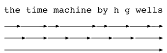
fig_truncated_bptt illustrates the three strategies when analyzing the first few characters of The Time Machine using backpropagation through time for RNNs:

• The first row is the randomized truncation that partitions the text into segments of varying lengths.
• The second row is the regular truncation that breaks the text into subsequences of the same length. This is what we have been doing in RNN experiments.
• The third row is the full backpropagation through time that leads to a computationally infeasible expression.

Unfortunately, while appealing in theory, randomized truncation does not work much better than regular truncation, most likely due to a number of factors. First, the effect of an observation after a number of backpropagation steps into the past is quite sufficient to capture dependencies in practice. Second, the increased variance counteracts the fact that the gradient is more accurate with more steps. Third, we actually want models that have only a short range of interactions. Hence, regularly truncated backpropagation through time has a slight regularizing effect that can be desirable.

Backpropagation Through Time in Detail

After discussing the general principle, let's discuss backpropagation through time in detail. In contrast to the analysis in subsec_bptt_analysis, in the following we will show how to compute the gradients of the objective function with respect to all the decomposed model parameters. To keep things simple, we consider an RNN without bias parameters, whose activation function in the hidden layer uses the identity mapping ($\phi(x)=x$). For time step $t$, let the single example input and the target be $\mathbf{x}_t \in \mathbb{R}^d$ and $y_t$, respectively. The hidden state $\mathbf{h}_t \in \mathbb{R}^h$ and the output $\mathbf{o}_t \in \mathbb{R}^q$ are computed as

$$\begin{aligned}\mathbf{h}_t &= \mathbf{W}_\textrm{hx} \mathbf{x}_t + \mathbf{W}_\textrm{hh} \mathbf{h}_{t-1},\\ \mathbf{o}_t &= \mathbf{W}_\textrm{qh} \mathbf{h}_{t},\end{aligned}$$

where $\mathbf{W}_\textrm{hx} \in \mathbb{R}^{h \times d}$, $\mathbf{W}_\textrm{hh} \in \mathbb{R}^{h \times h}$, and $\mathbf{W}_\textrm{qh} \in \mathbb{R}^{q \times h}$ are the weight parameters. Denote by $l(\mathbf{o}_t, y_t)$ the loss at time step $t$. Our objective function, the loss over $T$ time steps from the beginning of the sequence is thus

$L = \frac{1}{T} \sum_{t=1}^T l(\mathbf{o}_t, y_t).$

In order to visualize the dependencies among model variables and parameters during computation of the RNN, we can draw a computational graph for the model, as shown in fig_rnn_bptt. For example, the computation of the hidden states of time step 3, $\mathbf{h}_3$, depends on the model parameters $\mathbf{W}_\textrm{hx}$ and $\mathbf{W}_\textrm{hh}$, the hidden state of the previous time step $\mathbf{h}_2$, and the input of the current time step $\mathbf{x}_3$.

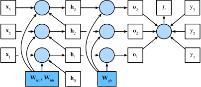
As just mentioned, the model parameters in fig_rnn_bptt are $\mathbf{W}_\textrm{hx}$, $\mathbf{W}_\textrm{hh}$, and $\mathbf{W}_\textrm{qh}$. Generally, training this model requires gradient computation with respect to these parameters $\partial L/\partial \mathbf{W}_\textrm{hx}$, $\partial L/\partial \mathbf{W}_\textrm{hh}$, and $\partial L/\partial \mathbf{W}_\textrm{qh}$. According to the dependencies in fig_rnn_bptt, we can traverse in the opposite direction of the arrows to calculate and store the gradients in turn. To flexibly express the multiplication of matrices, vectors, and scalars of different shapes in the chain rule, we continue to use the $\textrm{prod}$ operator as described in sec_backprop.

First of all, differentiating the objective function with respect to the model output at any time step $t$ is fairly straightforward:

$\frac{\partial L}{\partial \mathbf{o}_t} = \frac{\partial l (\mathbf{o}_t, y_t)}{T \cdot \partial \mathbf{o}_t} \in \mathbb{R}^q.$

Now we can calculate the gradient of the objective with respect to the parameter $\mathbf{W}_\textrm{qh}$ in the output layer: $\partial L/\partial \mathbf{W}_\textrm{qh} \in \mathbb{R}^{q \times h}$. Based on fig_rnn_bptt, the objective $L$ depends on $\mathbf{W}_\textrm{qh}$ via $\mathbf{o}_1, \ldots, \mathbf{o}_T$. Using the chain rule yields

$$\frac{\partial L}{\partial \mathbf{W}_\textrm{qh}} = \sum_{t=1}^T \textrm{prod}\left(\frac{\partial L}{\partial \mathbf{o}_t}, \frac{\partial \mathbf{o}_t}{\partial \mathbf{W}_\textrm{qh}}\right) = \sum_{t=1}^T \frac{\partial L}{\partial \mathbf{o}_t} \mathbf{h}_t^\top,$$

where $\partial L/\partial \mathbf{o}_t$ is given by eq_bptt_partial_L_ot.

Next, as shown in fig_rnn_bptt, at the final time step $T$, the objective function $L$ depends on the hidden state $\mathbf{h}_T$ only via $\mathbf{o}_T$. Therefore, we can easily find the gradient $\partial L/\partial \mathbf{h}_T \in \mathbb{R}^h$ using the chain rule:

$\frac{\partial L}{\partial \mathbf{h}_T} = \textrm{prod}\left(\frac{\partial L}{\partial \mathbf{o}_T}, \frac{\partial \mathbf{o}_T}{\partial \mathbf{h}_T} \right) = \mathbf{W}_\textrm{qh}^\top \frac{\partial L}{\partial \mathbf{o}_T}.$

It gets trickier for any time step $t < T$, where the objective function $L$ depends on $\mathbf{h}_t$ via $\mathbf{h}_{t+1}$ and $\mathbf{o}_t$. According to the chain rule, the gradient of the hidden state $\partial L/\partial \mathbf{h}_t \in \mathbb{R}^h$ at any time step $t < T$ can be recurrently computed as:

$\frac{\partial L}{\partial \mathbf{h}_t} = \textrm{prod}\left(\frac{\partial L}{\partial \mathbf{h}_{t+1}}, \frac{\partial \mathbf{h}_{t+1}}{\partial \mathbf{h}_t} \right) + \textrm{prod}\left(\frac{\partial L}{\partial \mathbf{o}_t}, \frac{\partial \mathbf{o}_t}{\partial \mathbf{h}_t} \right) = \mathbf{W}_\textrm{hh}^\top \frac{\partial L}{\partial \mathbf{h}_{t+1}} + \mathbf{W}_\textrm{qh}^\top \frac{\partial L}{\partial \mathbf{o}_t}.$

For analysis, expanding the recurrent computation for any time step $1 \leq t \leq T$ gives

$\frac{\partial L}{\partial \mathbf{h}_t}= \sum_{i=t}^T {\left(\mathbf{W}_\textrm{hh}^\top\right)}^{T-i} \mathbf{W}_\textrm{qh}^\top \frac{\partial L}{\partial \mathbf{o}_{T+t-i}}.$

We can see from eq_bptt_partial_L_ht that this simple linear example already exhibits some key problems of long sequence models: it involves potentially very large powers of $\mathbf{W}_\textrm{hh}^\top$. In it, eigenvalues smaller than 1 vanish and eigenvalues larger than 1 diverge. This is numerically unstable, which manifests itself in the form of vanishing and exploding gradients. One way to address this is to truncate the time steps at a computationally convenient size as discussed in subsec_bptt_analysis. In practice, this truncation can also be effected by detaching the gradient after a given number of time steps. Later on, we will see how more sophisticated sequence models such as long short-term memory can alleviate this further.

Finally, fig_rnn_bptt shows that the objective function $L$ depends on model parameters $\mathbf{W}_\textrm{hx}$ and $\mathbf{W}_\textrm{hh}$ in the hidden layer via hidden states $\mathbf{h}_1, \ldots, \mathbf{h}_T$. To compute gradients with respect to such parameters $\partial L / \partial \mathbf{W}_\textrm{hx} \in \mathbb{R}^{h \times d}$ and $\partial L / \partial \mathbf{W}_\textrm{hh} \in \mathbb{R}^{h \times h}$, we apply the chain rule giving

$$\begin{aligned} \frac{\partial L}{\partial \mathbf{W}_\textrm{hx}} &= \sum_{t=1}^T \textrm{prod}\left(\frac{\partial L}{\partial \mathbf{h}_t}, \frac{\partial \mathbf{h}_t}{\partial \mathbf{W}_\textrm{hx}}\right) = \sum_{t=1}^T \frac{\partial L}{\partial \mathbf{h}_t} \mathbf{x}_t^\top,\\ \frac{\partial L}{\partial \mathbf{W}_\textrm{hh}} &= \sum_{t=1}^T \textrm{prod}\left(\frac{\partial L}{\partial \mathbf{h}_t}, \frac{\partial \mathbf{h}_t}{\partial \mathbf{W}_\textrm{hh}}\right) = \sum_{t=1}^T \frac{\partial L}{\partial \mathbf{h}_t} \mathbf{h}_{t-1}^\top, \end{aligned}$$

where $\partial L/\partial \mathbf{h}_t$ which is recurrently computed by eq_bptt_partial_L_hT_final_step and eq_bptt_partial_L_ht_recur is the key quantity that affects the numerical stability.

Since backpropagation through time is the application of backpropagation in RNNs, as we have explained in sec_backprop, training RNNs alternates forward propagation with backpropagation through time. Moreover, backpropagation through time computes and stores the above gradients in turn. Specifically, stored intermediate values are reused to avoid duplicate calculations, such as storing $\partial L/\partial \mathbf{h}_t$ to be used in computation of both $\partial L / \partial \mathbf{W}_\textrm{hx}$ and $\partial L / \partial \mathbf{W}_\textrm{hh}$.

Summary

Backpropagation through time is merely an application of backpropagation to sequence models with a hidden state. Truncation, such as regular or randomized, is needed for computational convenience and numerical stability. High powers of matrices can lead to divergent or vanishing eigenvalues. This manifests itself in the form of exploding or vanishing gradients. For efficient computation, intermediate values are cached during backpropagation through time.

Exercises

1. Assume that we have a symmetric matrix $\mathbf{M} \in \mathbb{R}^{n \times n}$ with eigenvalues $\lambda_i$ whose corresponding eigenvectors are $\mathbf{v}_i$ ($i = 1, \ldots, n$). Without loss of generality, assume that they are ordered in the order $|\lambda_i| \geq |\lambda_{i+1}|$.
   1. Show that $\mathbf{M}^k$ has eigenvalues $\lambda_i^k$.
   2. Prove that for a random vector $\mathbf{x} \in \mathbb{R}^n$, with high probability $\mathbf{M}^k \mathbf{x}$ will be very much aligned with the eigenvector $\mathbf{v}_1$ of $\mathbf{M}$. Formalize this statement.
   3. What does the above result mean for gradients in RNNs?
2. Besides gradient clipping, can you think of any other methods to cope with gradient explosion in recurrent neural networks?

Discussions