(Optional) the Policy Gradient Theorem

In this optional section where we're going to study how we differentiate the objective function that we will use to approximate the policy gradient.

Let's first recap our different formulas:

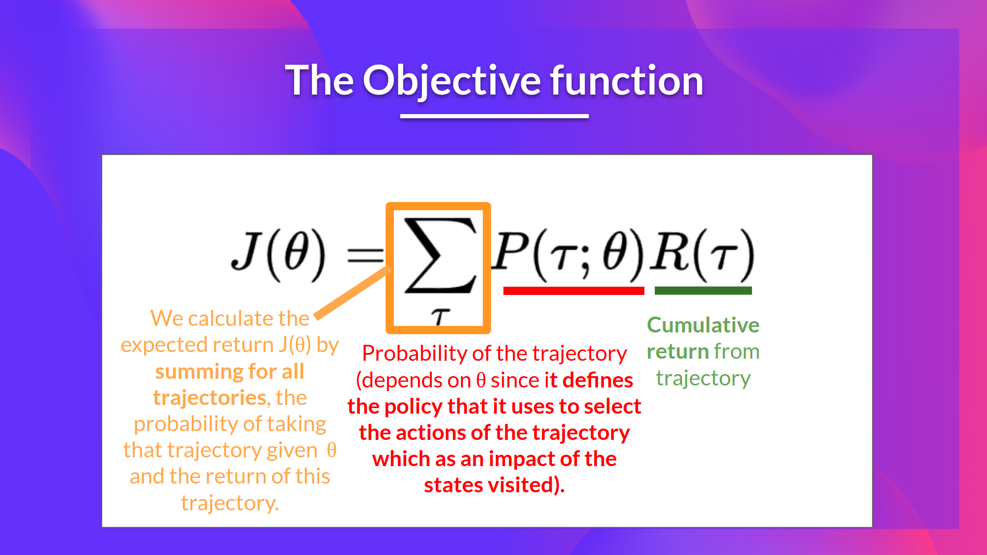
1. The Objective function

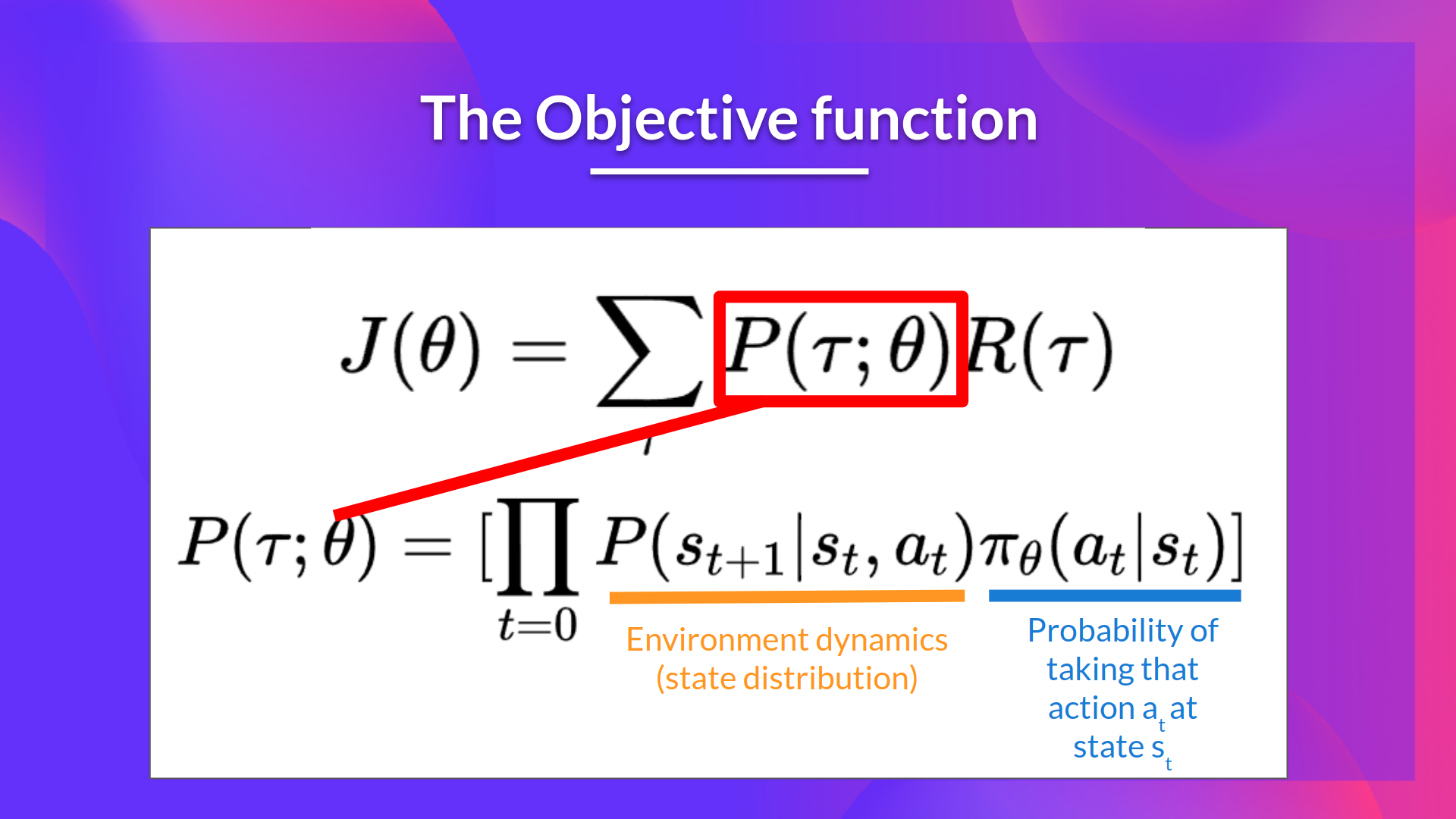
1. The probability of a trajectory (given that action comes from \(\pi_\theta\)):

So we have:

\(\nabla_\theta J(\theta) = \nabla_\theta \sum_{\tau}P(\tau;\theta)R(\tau)\)

We can rewrite the gradient of the sum as the sum of the gradient:

\( = \sum_{\tau} \nabla_\theta (P(\tau;\theta)R(\tau)) = \sum_{\tau} \nabla_\theta P(\tau;\theta)R(\tau) \) as \(R(\tau)\) is not dependent on \(\theta\)

We then multiply every term in the sum by \(\frac{P(\tau;\theta)}{P(\tau;\theta)}\)(which is possible since it's = 1)

\( = \sum_{\tau} \frac{P(\tau;\theta)}{P(\tau;\theta)}\nabla_\theta P(\tau;\theta)R(\tau) \)

We can simplify further this since \( \frac{P(\tau;\theta)}{P(\tau;\theta)}\nabla_\theta P(\tau;\theta) = P(\tau;\theta)\frac{\nabla_\theta P(\tau;\theta)}{P(\tau;\theta)} \).

Thus we can rewrite the sum as

\( P(\tau;\theta)\frac{\nabla_\theta P(\tau;\theta)}{P(\tau;\theta)}= \sum_{\tau} P(\tau;\theta) \frac{\nabla_\theta P(\tau;\theta)}{P(\tau;\theta)}R(\tau) \)

We can then use the derivative log trick (also called likelihood ratio trick or REINFORCE trick), a simple rule in calculus that implies that \( \nabla_x log f(x) = \frac{\nabla_x f(x)}{f(x)} \)

So given we have \(\frac{\nabla_\theta P(\tau;\theta)}{P(\tau;\theta)} \) we transform it as \(\nabla_\theta log P(\tau|\theta) \)

So this is our likelihood policy gradient:

\( \nabla_\theta J(\theta) = \sum_{\tau} P(\tau;\theta) \nabla_\theta log P(\tau;\theta) R(\tau) \)

Thanks for this new formula, we can estimate the gradient using trajectory samples (we can approximate the likelihood ratio policy gradient with sample-based estimate if you prefer).

\(\nabla_\theta J(\theta) = \frac{1}{m} \sum^{m}{i=1} \nabla\theta log P(\tau^{(i)};\theta)R(\tau^{(i)})\) where each \(\tau^{(i)}\) is a sampled trajectory.

But we still have some mathematics work to do there: we need to simplify \( \nabla_\theta log P(\tau|\theta) \)

We know that:

\(\nabla_\theta log P(\tau^{(i)};\theta)= \nabla_\theta log[ \mu(s_0) \prod_{t=0}^{H} P(s_{t+1}^{(i)}|s_{t}^{(i)}, a_{t}^{(i)}) \pi_\theta(a_{t}^{(i)}|s_{t}^{(i)})]\)

Where \(\mu(s_0)\) is the initial state distribution and \( P(s_{t+1}^{(i)}|s_{t}^{(i)}, a_{t}^{(i)}) \) is the state transition dynamics of the MDP.

We know that the log of a product is equal to the sum of the logs:

\(\nabla_\theta log P(\tau^{(i)};\theta)= \nabla_\theta \left[log \mu(s_0) + \sum\limits_{t=0}^{H}log P(s_{t+1}^{(i)}|s_{t}^{(i)} a_{t}^{(i)}) + \sum\limits_{t=0}^{H}log \pi_\theta(a_{t}^{(i)}|s_{t}^{(i)})\right] \)

We also know that the gradient of the sum is equal to the sum of gradient:

\( \nabla_\theta log P(\tau^{(i)};\theta)=\nabla_\theta log\mu(s_0) + \nabla_\theta \sum\limits_{t=0}^{H} log P(s_{t+1}^{(i)}|s_{t}^{(i)} a_{t}^{(i)}) + \nabla_\theta \sum\limits_{t=0}^{H} log \pi_\theta(a_{t}^{(i)}|s_{t}^{(i)}) \)

Since neither initial state distribution or state transition dynamics of the MDP are dependent of \(\theta\), the derivate of both terms are 0. So we can remove them:

Since: \(\nabla_\theta \sum_{t=0}^{H} log P(s_{t+1}^{(i)}|s_{t}^{(i)} a_{t}^{(i)}) = 0 \) and \( \nabla_\theta \mu(s_0) = 0\)

\(\nabla_\theta log P(\tau^{(i)};\theta) = \nabla_\theta \sum_{t=0}^{H} log \pi_\theta(a_{t}^{(i)}|s_{t}^{(i)})\)

We can rewrite the gradient of the sum as the sum of gradients:

\( \nabla_\theta log P(\tau^{(i)};\theta)= \sum_{t=0}^{H} \nabla_\theta log \pi_\theta(a_{t}^{(i)}|s_{t}^{(i)}) \)

So, the final formula for estimating the policy gradient is:

\( \nabla_{\theta} J(\theta) = \hat{g} = \frac{1}{m} \sum^{m}{i=1} \sum^{H}{t=0} \nabla_\theta \log \pi_\theta(a^{(i)}{t} | s{t}^{(i)})R(\tau^{(i)}) \)