
Chapter 48
08. Milestone Project 2: PyTorch Paper Replicating

08. Milestone Project 2: PyTorch Paper Replicating
The goal of machine learning research paper replicating is: turn a ML research paper into usable code.
In this notebook, we're going to be replicating the Vision Transformer (ViT) architecture/paper with PyTorch: https://arxiv.org/abs/2010.11929
See ground truth notebook here: https://www.learnpytorch.io/08_pytorch_paper_replicating/
0. Get setup
Let's import code we've previously written + required libraries.
# For this notebook to run with updated APIs, we need torch 1.12+ and torchvision 0.13+
try:
    import torch
    import torchvision
    assert int(torch.__version__.split(".")[1]) >= 12, "torch version should be 1.12+"
    assert int(torchvision.__version__.split(".")[1]) >= 13, "torchvision version should be 0.13+"
    print(f"torch version: {torch.__version__}")
    print(f"torchvision version: {torchvision.__version__}")
except:
    print(f"[INFO] torch/torchvision versions not as required, installing nightly versions.")
    !pip3 install -U --pre torch torchvision torchaudio --extra-index-url https://download.pytorch.org/whl/nightly/cu113
    import torch
    import torchvision
    print(f"torch version: {torch.__version__}")
    print(f"torchvision version: {torchvision.__version__}")
Output
torch version: 1.12.0+cu113
torchvision version: 0.13.0+cu113
# Continue with regular imports
import matplotlib.pyplot as plt
import torch
import torchvision

from torch import nn
from torchvision import transforms

# Try to get torchinfo, install it if it doesn't work
try:
    from torchinfo import summary
except:
    print("[INFO] Couldn't find torchinfo... installing it.")
    !pip install -q torchinfo
    from torchinfo import summary

# Try to import the going_modular directory, download it from GitHub if it doesn't work
try:
    from going_modular.going_modular import data_setup, engine
    from helper_functions import download_data, set_seeds, plot_loss_curves
except:
    # Get the going_modular scripts
    print("[INFO] Couldn't find going_modular or helper_functions scripts... downloading them from GitHub.")
    !git clone https://github.com/mrdbourke/pytorch-deep-learning
    !mv pytorch-deep-learning/going_modular .
    !mv pytorch-deep-learning/helper_functions.py . # get the helper_functions.py script
    !rm -rf pytorch-deep-learning
    from going_modular.going_modular import data_setup, engine
from helper_functions import download_data, set_seeds, plot_loss_curves# Setup device agnostic code
device = "cuda" if torch.cuda.is_available() else "cpu"
deviceOutput
'cuda'
1. Get data
The whole goal of what we're trying to do is to replicate the ViT architecture for our FoodVision Mini problem.
To do that, we need some data.
Namely, the pizza, steak and sushi images we've been using so far.
# Download pizza, steak, sushi images from GitHub
image_path = download_data(source="https://github.com/mrdbourke/pytorch-deep-learning/raw/main/data/pizza_steak_sushi.zip",
                           destination="pizza_steak_sushi")
image_path
Output
[INFO] data/pizza_steak_sushi directory exists, skipping download.
PosixPath('data/pizza_steak_sushi')# Setup directory paths to train and test images
train_dir = image_path / "train"
test_dir = image_path / "test"train_dir, test_dirOutput
(PosixPath('data/pizza_steak_sushi/train'),
 PosixPath('data/pizza_steak_sushi/test'))
2. Create Datasets and DataLoaders
from torchvision import transforms
from going_modular.going_modular import data_setup

# Create image size
IMG_SIZE = 224 # comes from Table 3 of the ViT paper

# Create transforms pipeline
manual_transforms = transforms.Compose([
                                        transforms.Resize((IMG_SIZE, IMG_SIZE)),
                                        transforms.ToTensor()
])

print(f"Manually created transforms: {manual_transforms}")
Output
Manually created transforms: Compose(
    Resize(size=(224, 224), interpolation=bilinear, max_size=None, antialias=None)
    ToTensor()
)
# Create a batch size of 32 (gthe paper uses 4096 but this may be too big for our smaller hardware... can always scale up later)
BATCH_SIZE = 32

# Create DataLoaders
train_dataloader, test_dataloader, class_names = data_setup.create_dataloaders(
    train_dir=train_dir,
    test_dir=test_dir,
    transform=manual_transforms,
    batch_size=BATCH_SIZE
)

len(train_dataloader), len(test_dataloader), class_names
Output
(8, 3, ['pizza', 'steak', 'sushi'])
2.3 Visualize a single a image
As always, let's adhere to the motto, visualize, visualize, visualize!
# Get a batch of images
image_batch, label_batch = next(iter(train_dataloader))

# Get a single image and label from the batch
image, label = image_batch[0], label_batch[0]

# View the single image and label shapes
image.shape, label
Output
(torch.Size([3, 224, 224]), tensor(0))
# Plot the image with matplotlib
import matplotlib.pyplot as plt

plt.imshow(image.permute(1, 2, 0)) # (color_channels, height, width) -> (height, width, color_channels)
plt.title(class_names[label])
plt.axis(False);
Output
<Figure size 432x288 with 1 Axes>
[省略较大 image/png 输出]
3. Replicating ViT: Overview
Looking at a whole machine learning research paper can be imtimidating.
So in order to make it more understandable, we can break it down into smaller pieces:
- Inputs - What goes into the model? (in our case, image tensors)
- Outputs - What comes out of the model/layer/block? (in our case, we want the model to output image classification labels)
- Layers - Takes an input, manipulates it with a function (for example could be self-attention).
- Blocks - A collection of layers.
- Model (or architecture) - A collection of blocks.
3.1 ViT overview: pieces of the puzzle
- Figure 1: Visual overview of the architecture
- Four equations: math equations which define the functions of each layer/block
- Table 1/3: different hyperparameters for the architecture/training.
- Text descriptions (especially section 3.1)
Figure 1
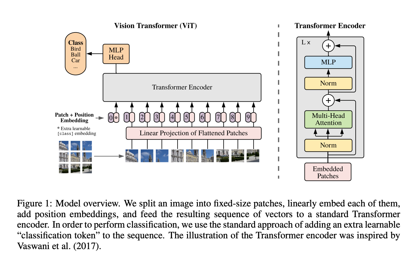
- Embedding = learnable representation (start with random numbers and improve over time)
Four equations

Section 3.1 describes the various equations:
Equation 1: An overview of the model is depicted in Figure 1. The standard Transformer receives as input a 1D sequence of token embeddings. To handle images, we reshape the image into a sequence of flattened patches , where is the resolution of the original image, is the number of channels, is the resolution of each image patch, and is the resulting number of patches, which also serves as the effective input sequence length for the Transformer. The Transformer uses constant latent vector size through all of its layers, so we flatten the patches and map to dimensions with a trainable linear projection (Eq. 1). We refer to the output of this projection as the patch embeddings.
Equation 1: Position embeddings are added to the patch embeddings to retain positional information. We use standard learnable position embeddings, since we have not observed significant performance gains from using more advanced 2D-aware position embeddings (Appendix D.4). The resulting sequence of embedding vectors serves as input to the encoder.
In pseudocode:
# Equation 1
x_input = [class_token, image_patch_1, image_patch_2, ... image_patch_N] + [class_token_pos, image_patch_1_pos, image_patch_2_pos, ... image_patch_N_pos]
Equations 2&3: The Transformer encoder (Vaswani et al., 2017) consists of alternating layers of multiheaded selfattention (MSA, see Appendix A) and MLP blocks (Eq. 2, 3). Layernorm (LN) is applied before every block, and residual connections after every block (Wang et al., 2019; Baevski & Auli, 2019).
In pseudocode:
# Equation 2
x_output_MSA_block = MSA_layer(LN_layer(x_input)) + x_input

# Equation 3
x_output_MLP_block = MLP_layer(LN_layer(x_output_MSA_block)) + x_output_MSA_block
Equation 4: Similar to BERT's [ class ] token, we prepend a learnable embedding to the sequence of embedded patches , whose state at the output of the Transformer encoder serves as the image representation y (Eq. 4). Both during pre-training and fine-tuning, a classification head is attached to . The classification head is implemented by a MLP with one hidden layer at pre-training time and by a single linear layer at fine-tuning time.
- MLP = multilayer perceptron = a neural network with X number of layers
- MLP = one hidden layer at training time
- MLP = single linear layer at fine-tuning time
In pseudocode:
# Equation 4
y = Linear_layer(LN_layer(x_output_MLP_block))
Table 1
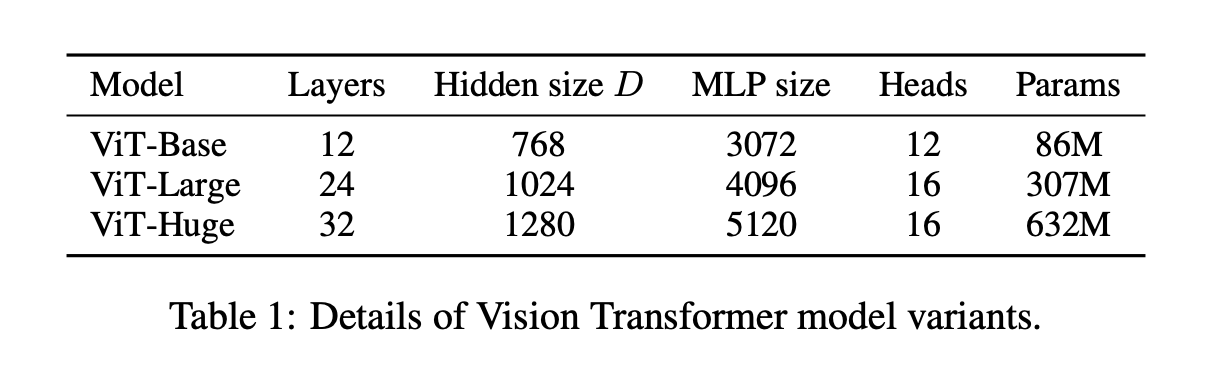
- ViT-Base, ViT-Large and ViT-Huge are all different sizes of the same model architecture
- ViT-B/16 = ViT-Base with image patch size 16x16
- Layers - the number of transformer encoder layers
- Hidden size - the embedding size throughout the architecture
- MLP size - the number of hidden units/neurons in the MLP
- Heads - the number of multi-head self-attention
4. Equation 1: Split data into patches and creating the class, position and patch embedding
Layers = input -> function -> output
What's the input shape?
What's the output shape?
- Input shape: (224, 224, 3) -> single image -> (height, width, color channels)
- Output shape: ???
4.1 Calculate input and output shapes by hand
Equation 1: An overview of the model is depicted in Figure 1. The standard Transformer receives as input a 1D sequence of token embeddings. To handle images, we reshape the image into a sequence of flattened patches , where is the resolution of the original image, is the number of channels, is the resolution of each image patch, and is the resulting number of patches, which also serves as the effective input sequence length for the Transformer. The Transformer uses constant latent vector size through all of its layers, so we flatten the patches and map to dimensions with a trainable linear projection (Eq. 1). We refer to the output of this projection as the patch embeddings.
Equation 1: Position embeddings are added to the patch embeddings to retain positional information. We use standard learnable position embeddings, since we have not observed significant performance gains from using more advanced 2D-aware position embeddings (Appendix D.4). The resulting sequence of embedding vectors serves as input to the encoder.
- Input shape: (height x width x color channels)
- Output shape:
- H = height
- W = width
- C = color channels
- P = patch size
- N = number of patches = (height * width) / p^2
- D = constant latent vector size = embedding dimension (see Table 1)
# Create example values
height = 224
width = 224
color_channels = 3
patch_size = 16

# Calculate the number of patches
number_of_patches = int((height * width) / patch_size**2)
number_of_patches
Output
196
# Input shape
embedding_layer_input_shape = (height, width, color_channels)

# Output shape
embedding_layer_output_shape = (number_of_patches, patch_size**2 * color_channels)

print(f"Input shape (single 2D image): {embedding_layer_input_shape}")
print(f"Output shape (single 1D sequence of patches): {embedding_layer_output_shape} -> (number_of_patches, embedding_dimension)")
Output
Input shape (single 2D image): (224, 224, 3)
Output shape (single 1D sequence of patches): (196, 768) -> (number_of_patches, embedding_dimension)
4.2 Turning a single image into patches
Let's visualize, visualize, visualize!
# View a single image
plt.imshow(image.permute(1, 2, 0))
plt.title(class_names[label])
plt.axis(False);
Output
<Figure size 432x288 with 1 Axes>
[省略较大 image/png 输出]
image.shapeOutput
torch.Size([3, 224, 224])
# Get the top row of the image
image_permuted = image.permute(1, 2, 0) # convert image to color channels last (H, W, C)

# Index to plot the top row of pixels
patch_size = 16
plt.figure(figsize=(patch_size, patch_size))
plt.imshow(image_permuted[:patch_size, :, :])
Output
<matplotlib.image.AxesImage at 0x7fc62c2838d0>
<Figure size 1152x1152 with 1 Axes>

# Setup code to plot top row as patches
img_size = 224
patch_size = 16
num_patches = img_size/patch_size
assert img_size % patch_size == 0, "Image size must be divisible by patch size"
print(f"Number of patches per row: {num_patches}\nPatch size: {patch_size} pixels x {patch_size} pixels")

# Create a series of subplots
fig, axs = plt.subplots(nrows=1,
                        ncols=img_size // patch_size, # one column for each patch
                        sharex=True,
                        sharey=True,
                        figsize=(patch_size, patch_size))

# Iterate through number of patches in the top row
for i, patch in enumerate(range(0, img_size, patch_size)):
  axs[i].imshow(image_permuted[:patch_size, patch:patch+patch_size, :]);
  axs[i].set_xlabel(i+1) # set the patch label
  axs[i].set_xticks([])
  axs[i].set_yticks([])
Output
Number of patches per row: 14.0
Patch size: 16 pixels x 16 pixels
<Figure size 1152x1152 with 14 Axes>

# Setup code to plot whole image as patches
img_size = 224
patch_size = 16
num_patches = img_size/patch_size
assert img_size % patch_size == 0, "Image size must be divisible by patch size"
print(f"Number of patches per row: {num_patches}\
  \nNumber of patches per column: {num_patches}\
  \nTotal patches: {num_patches*num_patches}\
  \nPatch size: {patch_size} pixels x {patch_size} pixels")

# Create a series of subplots
fig, axs = plt.subplots(nrows=img_size // patch_size,
                        ncols=img_size // patch_size,
                        figsize=(num_patches, num_patches),
                        sharex=True,
                        sharey=True)

# Loop through height and width of image
for i, patch_height in enumerate(range(0, img_size, patch_size)): # iterate through height
  for j, patch_width in enumerate(range(0, img_size, patch_size)):
    # Plot the permuted image on the different axes
    axs[i, j].imshow(image_permuted[patch_height:patch_height+patch_size, # iterate through height
                                    patch_width:patch_width+patch_size, # iterate through width
                                    :]) # get all color channels
    # Set up label information for each subplot (patch)
    axs[i, j].set_ylabel(i+1,
                         rotation="horizontal",
                         horizontalalignment="right",
                         verticalalignment="center")
    axs[i, j].set_xlabel(j+1)
    axs[i, j].set_xticks([])
    axs[i, j].set_yticks([])
    axs[i, j].label_outer()

# Set up a title for the plot
fig.suptitle(f"{class_names[label]} -> Patchified", fontsize=14)
plt.show()
Output
Number of patches per row: 14.0
Number of patches per column: 14.0
Total patches: 196.0
Patch size: 16 pixels x 16 pixels
<Figure size 1008x1008 with 196 Axes>
[省略较大 image/png 输出]
4.3 Creating image patches and turning them into patch embeddings
Perhaps we could create the image patches and image patch embeddings in a single step using torch.nn.Conv2d() and setting the kernel size and stride parameters to patch_size.
# Create conv2d layer to turn image into patches of learnable feature maps (embeddings)
from torch import nn

# Set the patch size
patch_size = 16

# Create a conv2d lyaer with hyperparameters from the ViT paper
conv2d = nn.Conv2d(in_channels=3, # for color images
                   out_channels=768, # D size from Table 1 for ViT-Base
                   kernel_size=patch_size,
                   stride=patch_size,
                   padding=0)
conv2d
Output
Conv2d(3, 768, kernel_size=(16, 16), stride=(16, 16))
# View single image
plt.imshow(image.permute(1, 2, 0))
plt.title(class_names[label])
plt.axis(False);
Output
<Figure size 432x288 with 1 Axes>
[省略较大 image/png 输出]
# Pass the image through the convolutional layer
image_out_of_conv = conv2d(image.unsqueeze(0)) # add batch dimension -> (batch_size, color_channels, height, width)
print(image_out_of_conv.shape)
Output
torch.Size([1, 768, 14, 14])
image_out_of_conv.requires_gradOutput
True
Now we've passed a single image to our conv2d layer, it's shape is:
torch.Size([1, 768, 14, 14]) # [batch_size, embedding_dim, feature_map_height, feature_map_width] # plot random convolutional feature maps (embeddings)
import random
random_indexes = random.sample(range(0, 758), k=5)
print(f"Showing random convolutional feature maps from indexes: {random_indexes}")
# Create plot
fig, axs = plt.subplots(nrows=1, ncols=5, figsize=(12, 12))
# Plot random image feature maps
for i, idx in enumerate(random_indexes):
image_conv_feature_map = image_out_of_conv[:, idx, :, :] # index on the output tensor of the conv2d layer
axs[i].imshow(image_conv_feature_map.squeeze().detach().numpy()) # remove batch dimension, and remove from grad tracking/switch to numpy for matplotlib
axs[i].set(xticklabels=[], yticklabels=[], xticks=[], yticks=[])Output
Showing random convolutional feature maps from indexes: [507, 71, 166, 241, 272]
<Figure size 864x864 with 5 Axes>

# Get a single feature map in tensor form
single_feature_map = image_out_of_conv[:, 0, :, :]
single_feature_map, single_feature_map.requires_grad
Output
(tensor([[[ 0.1407,  0.1090,  0.1021,  0.1104,  0.0994, -0.0023,  0.0833,
            0.0281,  0.0831,  0.0941,  0.0986,  0.0203,  0.0206, -0.0152],
          [ 0.0804,  0.1664,  0.1979, -0.0078, -0.3030, -0.0536, -0.2039,
           -0.0388, -0.0347, -0.1243, -0.1810, -0.0476,  0.1051,  0.0399],
          [-0.0716,  0.0355, -0.0671, -0.0396, -0.2541, -0.1525, -0.1335,
           -0.1575,  0.0895, -0.0103, -0.1282, -0.0114, -0.0942, -0.0481],
          [-0.1791, -0.1164, -0.1725, -0.0481, -0.0625, -0.0877, -0.1679,
           -0.0722, -0.1618, -0.0711, -0.0335,  0.1048,  0.1567,  0.1100],
          [ 0.0778, -0.2123, -0.0797, -0.1068, -0.0471, -0.0960,  0.0561,
           -0.0643, -0.0510, -0.0651, -0.0275, -0.0313, -0.1188, -0.0143],
          [-0.1055, -0.0940,  0.0829, -0.0087, -0.0778, -0.1851, -0.1613,
            0.1131,  0.0694, -0.1660, -0.2467,  0.0015,  0.1099,  0.1271],
          [-0.0018,  0.0883, -0.0462, -0.0074,  0.0591, -0.1006, -0.0257,
           -0.2168, -0.1621,  0.1588,  0.0712,  0.0631, -0.1775, -0.1007],
          [ 0.0357, -0.0580, -0.1732, -0.2045, -0.0843, -0.1670, -0.0618,
            0.0191,  0.0565, -0.1508,  0.0103,  0.0300,  0.1253,  0.0356],
          [-0.0979, -0.1481, -0.1128,  0.1911,  0.1118,  0.1514, -0.1875,
           -0.2145,  0.0742,  0.0809,  0.2035,  0.0928,  0.1184,  0.1298],
          [-0.0954, -0.1065, -0.1638, -0.0156,  0.0218, -0.1327, -0.1192,
           -0.1086, -0.1809, -0.0102, -0.1456,  0.0052, -0.0445,  0.0401],
          [-0.0196,  0.0171,  0.0129, -0.1425, -0.0151, -0.0344, -0.0826,
           -0.0653, -0.1250,  0.0047, -0.0196, -0.0445,  0.0677,  0.0581],
          [-0.0221, -0.0131, -0.0670, -0.1478, -0.0123,  0.0458,  0.0050,
           -0.0714, -0.0824, -0.0079, -0.0218,  0.0119, -0.1344, -0.0957],
          [-0.1727, -0.0127, -0.0364, -0.0090, -0.0312, -0.0084,  0.0170,
           -0.0113, -0.1140, -0.1092, -0.1072, -0.0010,  0.0080, -0.1315],
          [-0.1228, -0.1214, -0.1354, -0.0643, -0.1033, -0.1008, -0.1099,
           -0.0781, -0.0485, -0.1678, -0.1026, -0.0602, -0.0902,  0.0780]]],
        grad_fn=<SliceBackward0>), True)
4.4 Flattening the patch embedding with torch.nn.Flatten()
Right now we've a series of convolutional feature maps (patch embeddings) that we want to flatten into a sequence of patch embeddings to satisfy the input criteria of the ViT Transformer Encoder.
print(f"{image_out_of_conv.shape} -> (batch_size, embedding_dim, feature_map_height, feature_map_width)")Output
torch.Size([1, 768, 14, 14]) -> (batch_size, embedding_dim, feature_map_height, feature_map_width)
Want: (batch_size, number_of_patches, embedding_dim)
from torch import nn
flatten_layer = nn.Flatten(start_dim=2,
                           end_dim=3)

flatten_layer(image_out_of_conv).shape
Output
torch.Size([1, 768, 196])
# Put everything together
plt.imshow(image.permute(1, 2, 0))
plt.title(class_names[label])
plt.axis(False)
print(f"Original image shape: {image.shape}")

# Turn image into feature maps
image_out_of_conv = conv2d(image.unsqueeze(0)) # add batch dimension
print(f"Image feature map (patches) shape: {image_out_of_conv.shape}")

# Flatten the feature maps
image_out_of_conv_flattened = flatten_layer(image_out_of_conv)
print(f"Flattened image feature map shape: {image_out_of_conv_flattened.shape}")
Output
Original image shape: torch.Size([3, 224, 224])
Image feature map (patches) shape: torch.Size([1, 768, 14, 14])
Flattened image feature map shape: torch.Size([1, 768, 196])
<Figure size 432x288 with 1 Axes>
[省略较大 image/png 输出]
# Rearrange output of flattened layer
image_out_of_conv_flattened_permuted = image_out_of_conv_flattened.permute(0, 2, 1)
print(f"{image_out_of_conv_flattened_permuted.shape} -> (batch_size, number_of_patches, embedding_dimension)")
Output
torch.Size([1, 196, 768]) -> (batch_size, number_of_patches, embedding_dimension)
# Get a single flattened feature map
single_flattened_feature_map = image_out_of_conv_flattened_permuted[:, :, 0]

# Plot the flattened feature map visually
plt.figure(figsize=(22, 22))
plt.imshow(single_flattened_feature_map.detach().numpy())
plt.title(f"Flattened feature map shape: {single_flattened_feature_map.shape}")
plt.axis(False);
Output
<Figure size 1584x1584 with 1 Axes>

4.5 Turning the ViT patch embedding layer into a PyTorch module
We want this module to do a few things:
- Create a class called
PatchEmbeddingthat inherits fromnn.Module. - Initialize with appropriate hyperparameters, such as channels, embedding dimension, patch size.
- Create a layer to turn an image into embedded patches using
nn.Conv2d(). - Create a layer to flatten the feature maps of the output of the layer in 3.
- Define a
foward()that defines the forward computation (e.g. pass through layer from 3 and 4). - Make sure the output shape of the layer reflects the required output shape of the patch embedding.
# 1. Create a class called PatchEmbedding
class PatchEmbedding(nn.Module):
  # 2. Initilaize the layer with appropriate hyperparameters
  def __init__(self,
               in_channels:int=3,
               patch_size:int=16,
               embedding_dim:int=768): # from Table 1 for ViT-Base
    super().__init__()

    self.patch_size = patch_size

    # 3. Create a layer to turn an image into embedded patches
    self.patcher = nn.Conv2d(in_channels=in_channels,
                             out_channels=embedding_dim,
                             kernel_size=patch_size,
                             stride=patch_size,
                             padding=0)

    # 4. Create a layer to flatten feature map outputs of Conv2d
    self.flatten = nn.Flatten(start_dim=2,
                              end_dim=3)

  # 5. Define a forward method to define the forward computation steps
  def forward(self, x):
    # Create assertion to check that inputs are the correct shape
    image_resolution = x.shape[-1]
    assert image_resolution % patch_size == 0, f"Input image size must be divisible by patch size, image shape: {image_resolution}, patch size: {self.patch_size}"

    # Perform the forward pass
    x_patched = self.patcher(x)
    x_flattened = self.flatten(x_patched)
    # 6. Make the returned sequence embedding dimensions are in the right order (batch_size, number_of_patches, embedding_dimension)
return x_flattened.permute(0, 2, 1)set_seeds()
# Create an instance of patch embedding layer
patchify = PatchEmbedding(in_channels=3,
patch_size=16,
embedding_dim=768)
# Pass a single image through patch embedding layer
print(f"Input image size: {image.unsqueeze(0).shape}")
patch_embedded_image = patchify(image.unsqueeze(0)) # add an extra batch dimension
print(f"Output patch embedding sequence shape: {patch_embedded_image.shape}")Output
Input image size: torch.Size([1, 3, 224, 224])
Output patch embedding sequence shape: torch.Size([1, 196, 768])
rand_image_tensor = torch.randn(1, 3, 224, 224)
rand_image_tensor_bad = torch.randn(1, 3, 250, 250)

# patchify(rand_image_tensor_bad)
4.6 Creating the class token embedding
Want to: prepend a learnable class token to the start of the patch embedding.
patch_embedded_imageOutput
tensor([[[-0.7665,  0.1767, -0.2405,  ...,  0.6293, -0.3423,  0.3247],
         [-0.7299,  0.1911, -0.1953,  ...,  0.5647, -0.3340,  0.2806],
         [-0.7201,  0.1827, -0.1611,  ...,  0.5443, -0.3373,  0.2574],
         ...,
         [-0.5255,  0.0765, -0.0469,  ...,  0.3121, -0.3001,  0.2329],
         [-0.4847,  0.1029, -0.0593,  ...,  0.2676, -0.2530,  0.0827],
         [-0.2441,  0.1201, -0.3067,  ...,  0.2972, -0.1575,  0.0815]]],
grad_fn=<PermuteBackward0>)# Get the batch size and embedding dimension
batch_size = patch_embedded_image.shape[0]
embedding_dimension = patch_embedded_image.shape[-1]
batch_size, embedding_dimensionOutput
(1, 768)
# Create class token embedding as a learnable parameter that shares the same size as the embedding dimension (D)
class_token = nn.Parameter(torch.ones(batch_size, 1, embedding_dimension),
                           requires_grad=True)
class_token.shape
Output
torch.Size([1, 1, 768])
patch_embedded_image.shapeOutput
torch.Size([1, 196, 768])
# Add the class token embedding to the front of the patch embedding
patch_embedded_image_with_class_embedding = torch.cat((class_token, patch_embedded_image),
                                                      dim=1) # number_of_patches dimension

print(patch_embedded_image_with_class_embedding)
print(f"Sequence of patch embeddings with class token prepended shape: {patch_embedded_image_with_class_embedding.shape} -> (batch_size, class_token + number_of_patches, embedding_dim)")
Output
tensor([[[ 1.0000,  1.0000,  1.0000,  ...,  1.0000,  1.0000,  1.0000],
         [-0.7665,  0.1767, -0.2405,  ...,  0.6293, -0.3423,  0.3247],
         [-0.7299,  0.1911, -0.1953,  ...,  0.5647, -0.3340,  0.2806],
         ...,
         [-0.5255,  0.0765, -0.0469,  ...,  0.3121, -0.3001,  0.2329],
         [-0.4847,  0.1029, -0.0593,  ...,  0.2676, -0.2530,  0.0827],
         [-0.2441,  0.1201, -0.3067,  ...,  0.2972, -0.1575,  0.0815]]],
       grad_fn=<CatBackward0>)
Sequence of patch embeddings with class token prepended shape: torch.Size([1, 197, 768]) -> (batch_size, class_token + number_of_patches, embedding_dim)
4.7 Creating the position embedding
Want to: create a series of 1D learnable position embeddings and to add them to the sequence of patch embeddings.
# Calculate N (number_of_patches)
number_of_patches = int((height * width) / patch_size**2)

# Get the embedding dimension
embedding_dimension = patch_embedded_image_with_class_embedding.shape[-1]

# Create the learnable 1D position embedding
position_embedding = nn.Parameter(torch.ones(1,
                                             number_of_patches+1,
                                             embedding_dimension),
                                  requires_grad=True)

position_embedding, position_embedding.shape
Output
(Parameter containing:
 tensor([[[1., 1., 1.,  ..., 1., 1., 1.],
          [1., 1., 1.,  ..., 1., 1., 1.],
          [1., 1., 1.,  ..., 1., 1., 1.],
          ...,
          [1., 1., 1.,  ..., 1., 1., 1.],
          [1., 1., 1.,  ..., 1., 1., 1.],
          [1., 1., 1.,  ..., 1., 1., 1.]]], requires_grad=True),
torch.Size([1, 197, 768]))# View the sequence of patch embeddings with the prepended class embedding
patch_embedded_image_with_class_embedding, patch_embedded_image_with_class_embedding.shapeOutput
(tensor([[[ 1.0000,  1.0000,  1.0000,  ...,  1.0000,  1.0000,  1.0000],
          [-0.7665,  0.1767, -0.2405,  ...,  0.6293, -0.3423,  0.3247],
          [-0.7299,  0.1911, -0.1953,  ...,  0.5647, -0.3340,  0.2806],
          ...,
          [-0.5255,  0.0765, -0.0469,  ...,  0.3121, -0.3001,  0.2329],
          [-0.4847,  0.1029, -0.0593,  ...,  0.2676, -0.2530,  0.0827],
          [-0.2441,  0.1201, -0.3067,  ...,  0.2972, -0.1575,  0.0815]]],
grad_fn=<CatBackward0>), torch.Size([1, 197, 768]))# Add the position embedding to the patch and class token embedding
patch_and_position_embedding = patch_embedded_image_with_class_embedding + position_embedding
print(patch_and_position_embedding)
print(f"Patch and position embedding shape: {patch_and_position_embedding.shape}")Output
tensor([[[2.0000, 2.0000, 2.0000,  ..., 2.0000, 2.0000, 2.0000],
         [0.2335, 1.1767, 0.7595,  ..., 1.6293, 0.6577, 1.3247],
         [0.2701, 1.1911, 0.8047,  ..., 1.5647, 0.6660, 1.2806],
         ...,
         [0.4745, 1.0765, 0.9531,  ..., 1.3121, 0.6999, 1.2329],
         [0.5153, 1.1029, 0.9408,  ..., 1.2676, 0.7470, 1.0827],
         [0.7559, 1.1201, 0.6933,  ..., 1.2972, 0.8425, 1.0815]]],
       grad_fn=<AddBackward0>)
Patch and position embedding shape: torch.Size([1, 197, 768])
4.8 Putting it all together: from image to embedding
We've written code to turn an image into a flattened sequence of patch embeddings.
Now let's it all in one cell.
# Set seeds
set_seeds()

# 1. Set the patch size
patch_size = 16

# 2. Print shapes of the original image tensor and get the image dimensions
print(f"Image tensor shape: {image.shape}")
height, width = image.shape[1], image.shape[2]

# 3. Get image tensor and add a batch dimension
x = image.unsqueeze(0)
print(f"Input image shape: {x.shape}")

# 4. Create patch embedding layer
patch_embedding_layer = PatchEmbedding(in_channels=3,
                                       patch_size=patch_size,
                                       embedding_dim=768)

# 5. Pass input image through PatchEmbedding
patch_embedding = patch_embedding_layer(x)
print(f"Patch embedding shape: {patch_embedding.shape}")

# 6. Create class token embedding
batch_size = patch_embedding.shape[0]
embedding_dimension = patch_embedding.shape[-1]
class_token = nn.Parameter(torch.ones(batch_size, 1, embedding_dimension),
                           requires_grad=True) # make sure it's learnable
print(f"Class token embedding shape: {class_token.shape}")

# 7. Prepend the class token embedding to patch embedding
patch_embedding_class_token = torch.cat((class_token, patch_embedding), dim=1)
print(f"Patch embedding with class token shape: {patch_embedding_class_token.shape}")

# 8. Create position embedding
number_of_patches = int((height*width) / patch_size**2)
position_embedding = nn.Parameter(torch.ones(1, number_of_patches+1, embedding_dimension),
                                  requires_grad=True)

# 9. Add the position embedding to patch embedding with class token
patch_and_position_embedding = patch_embedding_class_token + position_embedding
print(f"Patch and position embedding shape: {patch_and_position_embedding.shape} ")
Output
Image tensor shape: torch.Size([3, 224, 224])
Input image shape: torch.Size([1, 3, 224, 224])
Patch embedding shape: torch.Size([1, 196, 768])
Class token embedding shape: torch.Size([1, 1, 768])
Patch embedding with class token shape: torch.Size([1, 197, 768])
Patch and position embedding shape: torch.Size([1, 197, 768])
5. Equation 2: Multihead Self-Attention (MSA block)
-
Multihead self-attention = which part of a sequence should pay the most attention to itself?
- In our case, we have a series of embedded image patches, which patch significantly relates to another patch.
- We want our neural network (ViT) to learn this relationship/representation.
-
To replicate MSA in PyTorch we can use: https://pytorch.org/docs/stable/generated/torch.nn.MultiheadAttention.html
-
LayerNorm = Layer normalization (LayerNorm) is a technique to normalize the distributions of intermediate layers. It enables smoother gradients, faster training, and better generalization accuracy.
- Normalization = make everything have the same mean and same standard deviation.
- In PyTorch = https://pytorch.org/docs/stable/generated/torch.nn.LayerNorm.html, normalizes values over dimension, in our case, the dimension is the embedding dimension.
- When we normalize along the embedding dimension, it's like making all of the stairs in a staircase the same size.
class MultiHeadSelfAttentionBlock(nn.Module):
  """Creates a multi-head self-attention block ("MSA block" for short).
  """
  def __init__(self,
               embedding_dim:int=768, # Hidden size D (embedding dimension) from Table 1 for ViT-Base
               num_heads:int=12, # Heads from Table 1 for ViT-Base
               attn_dropout:int=0):
    super().__init__()

    # Create the norm layer (LN)
    self.layer_norm = nn.LayerNorm(normalized_shape=embedding_dim)

    # Create multihead attention (MSA) layer
    self.multihead_attn = nn.MultiheadAttention(embed_dim=embedding_dim,
                                                num_heads=num_heads,
                                                dropout=attn_dropout,
                                                batch_first=True) # is the batch first? (batch, seq, feature) -> (batch, number_of_patches, embedding_dimension)

  def forward(self, x):
    x = self.layer_norm(x)
    attn_output, _ = self.multihead_attn(query=x,
                                         key=x,
                                         value=x,
                                         need_weights=False)
return attn_output# Create an instance MSA block
multihead_self_attention_block = MultiHeadSelfAttentionBlock(embedding_dim=768,
num_heads=12,
attn_dropout=0)
# Pass the patch and position image embedding sequence through MSA block
patched_image_through_msa_block = multihead_self_attention_block(patch_and_position_embedding)
print(f"Input shape of MSA block: {patch_and_position_embedding.shape}")
print(f"Output shape of MSA block: {patched_image_through_msa_block.shape}")Output
Input shape of MSA block: torch.Size([1, 197, 768])
Output shape of MSA block: torch.Size([1, 197, 768])
6. Equation 3: Multilayer Perceptron (MLP block)
- MLP = The MLP contains two layers with a GELU non-linearity (section 3.1).
- MLP = a quite broad term for a block with a series of layer(s), layers can be multiple or even only one hidden layer.
- Layers can mean: fully-connected, dense, linear, feed-forward, all are often similar names for the same thing. In PyTorch, they're often called
torch.nn.Linear()and in TensorFlow they might be calledtf.keras.layers.Dense() - GELU in PyTorch - https://pytorch.org/docs/stable/generated/torch.nn.GELU.html#torch.nn.GELU
- MLP number of hidden units = MLP Size in Table 1
- Dropout = Dropout, when used, is applied after
every dense layer except for the the qkv-projections and directly after adding positional- to patch
embeddings. Hybrid models are trained with the exact setup as their ViT counterparts.
- Value for Dropout available in Table 3
In pseudocode:
# MLP
x = linear -> non-linear -> dropout -> linear -> dropoutclass MLPBlock(nn.Module):
def __init__(self,
embedding_dim:int=768,
mlp_size:int=3072,
dropout:int=0.1):
super().__init__()
# Create the norm layer (LN)
self.layer_norm = nn.LayerNorm(normalized_shape=embedding_dim)
# Create the MLP
self.mlp = nn.Sequential(
nn.Linear(in_features=embedding_dim,
out_features=mlp_size),
nn.GELU(),
nn.Dropout(p=dropout),
nn.Linear(in_features=mlp_size,
out_features=embedding_dim),
nn.Dropout(p=dropout)
)
def forward(self, x):
x = self.layer_norm(x)
x = self.mlp(x)
return x
# return self.mlp(self.layer_norm(x)) # same as above # Create an instance of MLPBlock
mlp_block = MLPBlock(embedding_dim=768,
mlp_size=3072,
dropout=0.1)
# Pass output the MSABlock through MLPBlock
patched_image_through_mlp_block = mlp_block(patched_image_through_msa_block)
print(f"Input shape of MLP block: {patched_image_through_msa_block.shape}")
print(f"Output shape of MLP block: {patched_image_through_mlp_block.shape}")Output
Input shape of MLP block: torch.Size([1, 197, 768])
Output shape of MLP block: torch.Size([1, 197, 768])
7. Creating the Transformer Encoder
The Transformer Encoder is a combination of alternating blocks of MSA (equation 2) and MLP (equation 3).
And there are residual connections between each block.
- Encoder = turn a sequence into learnable representation
- Decoder = go from learn representation back to some sort of sequence
- Residual connections = add a layer(s) input to its subsequent output, this enables the creation of deeper networks (prevents weights from getting too small)
In pseudocode:
# Transformer Encoder
x_input -> MSA_block -> [MSA_block_output + x_input] -> MLP_block -> [MLP_block_output + MSA_block_output + x_input] -> ...
7.1 Create a custom Transformer Encoder block
class TransformerEncoderBlock(nn.Module):
  def __init__(self,
               embedding_dim:int=768, # Hidden size D from table 1, 768 for ViT-Base
               num_heads:int=12, # from table 1
               mlp_size:int=3072, # from table 1
               mlp_dropout:int=0.1, # from table 3
               attn_dropout:int=0):
    super().__init__()

    # Create MSA block (equation 2)
    self.msa_block = MultiHeadSelfAttentionBlock(embedding_dim=embedding_dim,
                                                 num_heads=num_heads,
                                                 attn_dropout=attn_dropout)

    # Create MLP block (equation 3)
    self.mlp_block = MLPBlock(embedding_dim=embedding_dim,
                              mlp_size=mlp_size,
                              dropout=mlp_dropout)

  def forward(self, x):
    x = self.msa_block(x) + x # residual/skip connection for equation 2
    x = self.mlp_block(x) + x # residual/skip connection for equation 3
return x # Create an instance of TransformerEncoderBlock()
transformer_encoder_block = TransformerEncoderBlock()
# Get a summary using torchinfo.summary
summary(model=transformer_encoder_block,
input_size=(1, 197, 768), # (batch_size, number_of_patches, embedding_dimension)
col_names=["input_size", "output_size", "num_params", "trainable"],
col_width=20,
row_settings=["var_names"])Output
============================================================================================================================================
Layer (type (var_name))                                      Input Shape          Output Shape         Param #              Trainable
============================================================================================================================================
TransformerEncoderBlock (TransformerEncoderBlock)            [1, 197, 768]        [1, 197, 768]        --                   True
├─MultiHeadSelfAttentionBlock (msa_block)                    [1, 197, 768]        [1, 197, 768]        --                   True
│    └─LayerNorm (layer_norm)                                [1, 197, 768]        [1, 197, 768]        1,536                True
│    └─MultiheadAttention (multihead_attn)                   --                   [1, 197, 768]        1,771,776            True
│    │    └─NonDynamicallyQuantizableLinear (out_proj)       --                   --                   590,592              True
├─MLPBlock (mlp_block)                                       [1, 197, 768]        [1, 197, 768]        --                   True
│    └─LayerNorm (layer_norm)                                [1, 197, 768]        [1, 197, 768]        1,536                True
│    └─Sequential (mlp)                                      [1, 197, 768]        [1, 197, 768]        --                   True
│    │    └─Linear (0)                                       [1, 197, 768]        [1, 197, 3072]       2,362,368            True
│    │    └─GELU (1)                                         [1, 197, 3072]       [1, 197, 3072]       --                   --
│    │    └─Dropout (2)                                      [1, 197, 3072]       [1, 197, 3072]       --                   --
│    │    └─Linear (3)                                       [1, 197, 3072]       [1, 197, 768]        2,360,064            True
│    │    └─Dropout (4)                                      [1, 197, 768]        [1, 197, 768]        --                   --
============================================================================================================================================
Total params: 7,087,872
Trainable params: 7,087,872
Non-trainable params: 0
Total mult-adds (M): 4.73
============================================================================================================================================
Input size (MB): 0.61
Forward/backward pass size (MB): 8.47
Params size (MB): 21.26
Estimated Total Size (MB): 30.34
============================================================================================================================================
7.2 Create a Transformer Encoder layer with in-built PyTorch layers
So far we've created a transformer encoder by hand.
But because of how good the Transformer architecture is, PyTorch has implemented ready to use Transformer Encoder layers: https://pytorch.org/docs/stable/nn.html#transformer-layers
We can create a Transformer Encoder with pure PyTorch layers: https://pytorch.org/docs/stable/generated/torch.nn.TransformerEncoderLayer.html#torch.nn.TransformerEncoderLayer
# Create the same as above with torch.nn.TransformerEncoderLayer()
torch_transformer_encoder_layer = nn.TransformerEncoderLayer(d_model=768, # embedding size from table 1
                                                             nhead=12, # heads from table 1
                                                             dim_feedforward=3072, # MLP size from table
                                                             dropout=0.1,
                                                             activation="gelu",
                                                             batch_first=True,
                                                             norm_first=True)

torch_transformer_encoder_layer
Output
TransformerEncoderLayer(
  (self_attn): MultiheadAttention(
    (out_proj): NonDynamicallyQuantizableLinear(in_features=768, out_features=768, bias=True)
  )
  (linear1): Linear(in_features=768, out_features=3072, bias=True)
  (dropout): Dropout(p=0.1, inplace=False)
  (linear2): Linear(in_features=3072, out_features=768, bias=True)
  (norm1): LayerNorm((768,), eps=1e-05, elementwise_affine=True)
  (norm2): LayerNorm((768,), eps=1e-05, elementwise_affine=True)
  (dropout1): Dropout(p=0.1, inplace=False)
  (dropout2): Dropout(p=0.1, inplace=False)
)# Get a summary using torchinfo.summary
summary(model=torch_transformer_encoder_layer,
input_size=(1, 197, 768), # (batch_size, number_of_patches, embedding_dimension)
col_names=["input_size", "output_size", "num_params", "trainable"],
col_width=20,
row_settings=["var_names"])Output
==================================================================================================================================
Layer (type (var_name))                            Input Shape          Output Shape         Param #              Trainable
==================================================================================================================================
TransformerEncoderLayer (TransformerEncoderLayer)  [1, 197, 768]        [1, 197, 768]        3,072                True
├─LayerNorm (norm1)                                [1, 197, 768]        [1, 197, 768]        (recursive)          True
├─MultiheadAttention (self_attn)                   [1, 197, 768]        [1, 197, 768]        2,362,368            True
├─Dropout (dropout1)                               [1, 197, 768]        [1, 197, 768]        --                   --
├─LayerNorm (norm2)                                [1, 197, 768]        [1, 197, 768]        (recursive)          True
├─Linear (linear1)                                 [1, 197, 768]        [1, 197, 3072]       2,362,368            True
├─LayerNorm (norm1)                                [1, 197, 768]        [1, 197, 768]        (recursive)          True
├─LayerNorm (norm2)                                [1, 197, 768]        [1, 197, 768]        (recursive)          True
├─Dropout (dropout)                                [1, 197, 3072]       [1, 197, 3072]       --                   --
├─Dropout (dropout2)                               [1, 197, 768]        [1, 197, 768]        --                   --
├─Linear (linear2)                                 [1, 197, 3072]       [1, 197, 768]        2,360,064            True
├─Dropout (dropout2)                               [1, 197, 768]        [1, 197, 768]        --                   --
==================================================================================================================================
Total params: 7,087,872
Trainable params: 7,087,872
Non-trainable params: 0
Total mult-adds (M): 4.73
==================================================================================================================================
Input size (MB): 0.61
Forward/backward pass size (MB): 6.05
Params size (MB): 18.89
Estimated Total Size (MB): 25.55
==================================================================================================================================
Why spend all this time recreating the transformer encoder when we could've just made it with a single PyTorch layer?
Practice. Practice. Practice.
Now we know how things are implemented behind the scenes, we can tweak them if necessary.
What are the benefits of using a pre-built PyTorch layer?
- Less prone to errors (goes through a bunch of testing)
- Potential benefit of speed ups (performance boosts)
8. Putting it all together to create ViT
# Create a ViT class
class ViT(nn.Module):
  def __init__(self,
               img_size:int=224, # Table 3 from the ViT paper
               in_channels:int=3,
               patch_size:int=16,
               num_transformer_layers:int=12, # Table 1 for "Layers" for ViT-Base
               embedding_dim:int=768, # Hidden size D from Table 1 for ViT-Base
               mlp_size:int=3072, # Table 1
               num_heads:int=12, # Table 1
               attn_dropout:int=0,
               mlp_dropout:int=0.1,
               embedding_dropout:int=0.1, # Dropout for patch and position embeddings
               num_classes:int=1000): # number of classes in our classification problem
    super().__init__()

    # Make an assertion that the image size is compatible with the patch size
    assert img_size % patch_size == 0,  f"Image size must be divisible by patch size, image: {img_size}, patch size: {patch_size}"

    # Calculate the number of patches (height * width/patch^2)
    self.num_patches = (img_size * img_size) // patch_size**2

    # Create learnable class embedding (needs to go at front of sequence of patch embeddings)
    self.class_embedding = nn.Parameter(data=torch.randn(1, 1, embedding_dim),
                                        requires_grad=True)

    # Create learnable position embedding
    self.position_embedding = nn.Parameter(data=torch.randn(1, self.num_patches+1, embedding_dim))

    # Create embedding dropout value
    self.embedding_dropout = nn.Dropout(p=embedding_dropout)

    # Create patch embedding layer
    self.patch_embedding = PatchEmbedding(in_channels=in_channels,
                                          patch_size=patch_size,
                                          embedding_dim=embedding_dim)

    # Create the Transformer Encoder block
    self.transformer_encoder = nn.Sequential(*[TransformerEncoderBlock(embedding_dim=embedding_dim,
                                                                       num_heads=num_heads,
                                                                       mlp_size=mlp_size,
                                                                       mlp_dropout=mlp_dropout) for _ in range(num_transformer_layers)])

    # Create classifier head
    self.classifier = nn.Sequential(
        nn.LayerNorm(normalized_shape=embedding_dim),
        nn.Linear(in_features=embedding_dim,
                  out_features=num_classes)
    )

  def forward(self, x):
    # Get the batch size
    batch_size = x.shape[0]

    # Create class token embedding and expand it to match the batch size (equation 1)
    class_token = self.class_embedding.expand(batch_size, -1, -1) # "-1" means to infer the dimensions

    # Create the patch embedding (equation 1)
    x = self.patch_embedding(x)

    # Concat class token embedding and patch embedding (equation 1)
    x = torch.cat((class_token, x), dim=1) # (batch_size, number_of_patches, embedding_dim)

    # Add position embedding to class token and patch embedding
    x = self.position_embedding + x

    # Apply dropout to patch embedding ("directly after adding positional- to patch embeddings")
    x = self.embedding_dropout(x)

    # Pass position and patch embedding to Transformer Encoder (equation 2 & 3)
    x = self.transformer_encoder(x)

    # Put 0th index logit through classifier (equation 4)
    x = self.classifier(x[:, 0])

return x batch_size=32
embedding_dim=768
class_embedding = nn.Parameter(data=torch.randn(1, 1, embedding_dim),
requires_grad=True)
class_embedding_expanded = class_embedding.expand(batch_size, -1, -1)
print(class_embedding.shape)
print(class_embedding_expanded.shape)Output
torch.Size([1, 1, 768])
torch.Size([32, 1, 768])
set_seeds()

# Create a random image tensor with same shape as a single image
random_image_tensor = torch.randn(1, 3, 224, 224)

# Create an instance of ViT with the number of classes we're working with (pizza, steak and sushi)
vit = ViT(num_classes=len(class_names))

# Pass the random image tensor to our ViT instance
vit(random_image_tensor)
Output
tensor([[-0.2377, 0.7360, 1.2137]], grad_fn=<AddmmBackward0>)
8.1 Getting a visual summary of our ViT model
from torchinfo import summary

summary(model=ViT(num_classes=len(class_names)),
        input_size=(1, 3, 224, 224), # (batch_size, color_channels, height, width)
        col_names=["input_size", "output_size", "num_params", "trainable"],
        col_width=20,
        row_settings=["var_names"])
Output
======================================================================================================================================================
Layer (type (var_name))                                                Input Shape          Output Shape         Param #              Trainable
======================================================================================================================================================
ViT (ViT)                                                              [1, 3, 224, 224]     [1, 3]               152,064              True
├─Dropout (embedding_dropout)                                          [1, 197, 768]        [1, 197, 768]        --                   --
├─PatchEmbedding (patch_embedding)                                     [1, 3, 224, 224]     [1, 196, 768]        --                   True
│    └─Conv2d (patcher)                                                [1, 3, 224, 224]     [1, 768, 14, 14]     590,592              True
│    └─Flatten (flatten)                                               [1, 768, 14, 14]     [1, 768, 196]        --                   --
├─Dropout (embedding_dropout)                                          [1, 197, 768]        [1, 197, 768]        --                   --
├─Sequential (transformer_encoder)                                     [1, 197, 768]        [1, 197, 768]        --                   True
│    └─TransformerEncoderBlock (0)                                     [1, 197, 768]        [1, 197, 768]        --                   True
│    │    └─MultiHeadSelfAttentionBlock (msa_block)                    [1, 197, 768]        [1, 197, 768]        2,363,904            True
│    │    └─MLPBlock (mlp_block)                                       [1, 197, 768]        [1, 197, 768]        4,723,968            True
│    └─TransformerEncoderBlock (1)                                     [1, 197, 768]        [1, 197, 768]        --                   True
│    │    └─MultiHeadSelfAttentionBlock (msa_block)                    [1, 197, 768]        [1, 197, 768]        2,363,904            True
│    │    └─MLPBlock (mlp_block)                                       [1, 197, 768]        [1, 197, 768]        4,723,968            True
│    └─TransformerEncoderBlock (2)                                     [1, 197, 768]        [1, 197, 768]        --                   True
│    │    └─MultiHeadSelfAttentionBlock (msa_block)                    [1, 197, 768]        [1, 197, 768]        2,363,904            True
│    │    └─MLPBlock (mlp_block)                                       [1, 197, 768]        [1, 197, 768]        4,723,968            True
│    └─TransformerEncoderBlock (3)                                     [1, 197, 768]        [1, 197, 768]        --                   True
│    │    └─MultiHeadSelfAttentionBlock (msa_block)                    [1, 197, 768]        [1, 197, 768]        2,363,904            True
│    │    └─MLPBlock (mlp_block)                                       [1, 197, 768]        [1, 197, 768]        4,723,968            True
│    └─TransformerEncoderBlock (4)                                     [1, 197, 768]        [1, 197, 768]        --                   True
│    │    └─MultiHeadSelfAttentionBlock (msa_block)                    [1, 197, 768]        [1, 197, 768]        2,363,904            True
│    │    └─MLPBlock (mlp_block)                                       [1, 197, 768]        [1, 197, 768]        4,723,968            True
│    └─TransformerEncoderBlock (5)                                     [1, 197, 768]        [1, 197, 768]        --                   True
│    │    └─MultiHeadSelfAttentionBlock (msa_block)                    [1, 197, 768]        [1, 197, 768]        2,363,904            True
│    │    └─MLPBlock (mlp_block)                                       [1, 197, 768]        [1, 197, 768]        4,723,968            True
│    └─TransformerEncoderBlock (6)                                     [1, 197, 768]        [1, 197, 768]        --                   True
│    │    └─MultiHeadSelfAttentionBlock (msa_block)                    [1, 197, 768]        [1, 197, 768]        2,363,904            True
│    │    └─MLPBlock (mlp_block)                                       [1, 197, 768]        [1, 197, 768]        4,723,968            True
│    └─TransformerEncoderBlock (7)                                     [1, 197, 768]        [1, 197, 768]        --                   True
│    │    └─MultiHeadSelfAttentionBlock (msa_block)                    [1, 197, 768]        [1, 197, 768]        2,363,904            True
│    │    └─MLPBlock (mlp_block)                                       [1, 197, 768]        [1, 197, 768]        4,723,968            True
│    └─TransformerEncoderBlock (8)                                     [1, 197, 768]        [1, 197, 768]        --                   True
│    │    └─MultiHeadSelfAttentionBlock (msa_block)                    [1, 197, 768]        [1, 197, 768]        2,363,904            True
│    │    └─MLPBlock (mlp_block)                                       [1, 197, 768]        [1, 197, 768]        4,723,968            True
│    └─TransformerEncoderBlock (9)                                     [1, 197, 768]        [1, 197, 768]        --                   True
│    │    └─MultiHeadSelfAttentionBlock (msa_block)                    [1, 197, 768]        [1, 197, 768]        2,363,904            True
│    │    └─MLPBlock (mlp_block)                                       [1, 197, 768]        [1, 197, 768]        4,723,968            True
│    └─TransformerEncoderBlock (10)                                    [1, 197, 768]        [1, 197, 768]        --                   True
│    │    └─MultiHeadSelfAttentionBlock (msa_block)                    [1, 197, 768]        [1, 197, 768]        2,363,904            True
│    │    └─MLPBlock (mlp_block)                                       [1, 197, 768]        [1, 197, 768]        4,723,968            True
│    └─TransformerEncoderBlock (11)                                    [1, 197, 768]        [1, 197, 768]        --                   True
│    │    └─MultiHeadSelfAttentionBlock (msa_block)                    [1, 197, 768]        [1, 197, 768]        2,363,904            True
│    │    └─MLPBlock (mlp_block)                                       [1, 197, 768]        [1, 197, 768]        4,723,968            True
├─Sequential (classifier)                                              [1, 768]             [1, 3]               --                   True
│    └─LayerNorm (0)                                                   [1, 768]             [1, 768]             1,536                True
│    └─Linear (1)                                                      [1, 768]             [1, 3]               2,307                True
======================================================================================================================================================
Total params: 85,800,963
Trainable params: 85,800,963
Non-trainable params: 0
Total mult-adds (M): 172.47
======================================================================================================================================================
Input size (MB): 0.60
Forward/backward pass size (MB): 102.88
Params size (MB): 257.55
Estimated Total Size (MB): 361.03
======================================================================================================================================================
 # Number of parameters in pretrained ViT
 num_params = 85,800,963
 num_params
Output
(85, 800, 963)
9. Setting up training code for our custom ViT
We've replicated the ViT architecture, now let's see how it performs on our FoodVision Mini data.
9.1 Creating an optimizer
The paper states it uses the Adam optimizer (section 4, Training & fine-tuning) with value of 0.9, of 0.999 (defaults) and a weight decay of 0.1.
Weight decay = Weight decay is a regularization technique by adding a small penalty, usually the L2 norm of the weights (all the weights of the model), to the loss function.
Regularization technique = prevents overfitting.
# vit9.2 Creating a loss function
The ViT paper doesn't actually mention what loss function they used.
So since it's a multi-class classification we'll use the torch.nn.CrossEntropyLoss().
9.3 Training our ViT Model
deviceOutput
'cuda'
from going_modular.going_modular import engine

set_seeds()

optimizer = torch.optim.Adam(vit.parameters(),
                             lr=1e-3,
                             betas=(0.9, 0.999),
                             weight_decay=0.1)

loss_fn = torch.nn.CrossEntropyLoss()

results = engine.train(model=vit,
                       train_dataloader=train_dataloader,
                       test_dataloader=test_dataloader,
                       epochs=10,
                       optimizer=optimizer,
                       loss_fn=loss_fn,
                       device=device)
Output
0%| | 0/10 [00:00<?, ?it/s]
Epoch: 1 | train_loss: 4.9009 | train_acc: 0.2969 | test_loss: 1.0362 | test_acc: 0.5417
Epoch: 2 | train_loss: 1.5928 | train_acc: 0.2773 | test_loss: 1.5662 | test_acc: 0.1979
Epoch: 3 | train_loss: 1.4393 | train_acc: 0.2617 | test_loss: 1.2755 | test_acc: 0.1979
Epoch: 4 | train_loss: 1.2928 | train_acc: 0.2891 | test_loss: 1.6844 | test_acc: 0.1979
Epoch: 5 | train_loss: 1.2678 | train_acc: 0.2852 | test_loss: 1.7159 | test_acc: 0.2604
Epoch: 6 | train_loss: 1.1954 | train_acc: 0.4102 | test_loss: 1.9489 | test_acc: 0.1979
Epoch: 7 | train_loss: 1.1835 | train_acc: 0.4062 | test_loss: 3.0747 | test_acc: 0.1979
Epoch: 8 | train_loss: 1.3447 | train_acc: 0.4180 | test_loss: 1.9179 | test_acc: 0.2604
Epoch: 9 | train_loss: 1.5294 | train_acc: 0.2383 | test_loss: 1.4440 | test_acc: 0.5417
Epoch: 10 | train_loss: 1.4364 | train_acc: 0.3359 | test_loss: 1.2803 | test_acc: 0.2604
9.4 What our training setup is missing
How is our training setup different to the ViT paper?
We've replicated model archirecture correctly.
But what was different between our training procedure (to get such poor results) and the ViT paper training procedure to get such great results?
The main things our training implementation is missing:
Prevent underfitting:
- Data - our setup uses far less data (225 vs millions)
Prevent overfitting:
- Learning rate warmup - start with a low learning rate and increase to a base LR
- Learning rate decay - as your model gets closer to convergence, start to lower the learning rate
- Gradient clipping - prevent gradients from getting too big
Search "pytorch [technique name]"
9.5 Plotting loss curves for our model
from helper_functions import plot_loss_curves

plot_loss_curves(results)
Output
<Figure size 1080x504 with 2 Axes>

Hmm it looks like our model is underfitting and overfitting... I wonder what techniques we could use to take care of both at the same time?
See more here: https://www.learnpytorch.io/04_pytorch_custom_datasets/#8-what-should-an-ideal-loss-curve-look-like
10. Using a pretrained ViT from torchvision.models
Generally, in deep learning if you can use a pretrained model from a large dataset on your own problem, it's often a good place to start.
If you can find a pretrained model and use transfer learning, give it a go, it often achieves great results with little data.
10.1 Why use a pretrained model?
- Sometimes data is limited
- Limited training resources
- Get better results faster (sometimes)...
# Cost of a TPUv3 for 30 days
cost = 30*24*8
print(f"Cost of renting a TPUv3 for 30 straight days: ${cost}USD")
Output
Cost of renting a TPUv3 for 30 straight days: $5760USD
# The following requires torch v0.12+ and torchvision 0.13+
import torch
import torchvision
print(torch.__version__)
print(torchvision.__version__)
Output
1.12.0+cu113
0.13.0+cu113
device = "cuda" if torch.cuda.is_available() else "cpu"
device
Output
'cuda'
10.2 Prepare a pretrained ViT for use with FoodVision Mini (turn it into a feature extractor)
# Get pretrained weights for ViT-Base
pretrained_vit_weights = torchvision.models.ViT_B_16_Weights.DEFAULT # "DEFAULT" = best available

# Setup a ViT model instance with pretrained weights
pretrained_vit = torchvision.models.vit_b_16(weights=pretrained_vit_weights).to(device)

# Freeze the base parameters
for parameter in pretrained_vit.parameters():
  parameter.requires_grad = False

# Update the classifier head
set_seeds()
pretrained_vit.heads = nn.Linear(in_features=768, out_features=len(class_names)).to(device)from torchinfo import summary
summary(model=pretrained_vit,
input_size=(1, 3, 224, 224), # (batch_size, color_channels, height, width)
col_names=["input_size", "output_size", "num_params", "trainable"],
col_width=20,
row_settings=["var_names"])Output
======================================================================================================================================================
Layer (type (var_name))                                                Input Shape          Output Shape         Param #              Trainable
======================================================================================================================================================
VisionTransformer (VisionTransformer)                                  [1, 3, 224, 224]     [1, 3]               768                  Partial
├─Conv2d (conv_proj)                                                   [1, 3, 224, 224]     [1, 768, 14, 14]     (590,592)            False
├─Encoder (encoder)                                                    [1, 197, 768]        [1, 197, 768]        151,296              False
│    └─Dropout (dropout)                                               [1, 197, 768]        [1, 197, 768]        --                   --
│    └─Sequential (layers)                                             [1, 197, 768]        [1, 197, 768]        --                   False
│    │    └─EncoderBlock (encoder_layer_0)                             [1, 197, 768]        [1, 197, 768]        (7,087,872)          False
│    │    └─EncoderBlock (encoder_layer_1)                             [1, 197, 768]        [1, 197, 768]        (7,087,872)          False
│    │    └─EncoderBlock (encoder_layer_2)                             [1, 197, 768]        [1, 197, 768]        (7,087,872)          False
│    │    └─EncoderBlock (encoder_layer_3)                             [1, 197, 768]        [1, 197, 768]        (7,087,872)          False
│    │    └─EncoderBlock (encoder_layer_4)                             [1, 197, 768]        [1, 197, 768]        (7,087,872)          False
│    │    └─EncoderBlock (encoder_layer_5)                             [1, 197, 768]        [1, 197, 768]        (7,087,872)          False
│    │    └─EncoderBlock (encoder_layer_6)                             [1, 197, 768]        [1, 197, 768]        (7,087,872)          False
│    │    └─EncoderBlock (encoder_layer_7)                             [1, 197, 768]        [1, 197, 768]        (7,087,872)          False
│    │    └─EncoderBlock (encoder_layer_8)                             [1, 197, 768]        [1, 197, 768]        (7,087,872)          False
│    │    └─EncoderBlock (encoder_layer_9)                             [1, 197, 768]        [1, 197, 768]        (7,087,872)          False
│    │    └─EncoderBlock (encoder_layer_10)                            [1, 197, 768]        [1, 197, 768]        (7,087,872)          False
│    │    └─EncoderBlock (encoder_layer_11)                            [1, 197, 768]        [1, 197, 768]        (7,087,872)          False
│    └─LayerNorm (ln)                                                  [1, 197, 768]        [1, 197, 768]        (1,536)              False
├─Linear (heads)                                                       [1, 768]             [1, 3]               2,307                True
======================================================================================================================================================
Total params: 85,800,963
Trainable params: 2,307
Non-trainable params: 85,798,656
Total mult-adds (M): 172.47
======================================================================================================================================================
Input size (MB): 0.60
Forward/backward pass size (MB): 104.09
Params size (MB): 257.55
Estimated Total Size (MB): 362.24
======================================================================================================================================================
10.3 Preparing data for the pretrained ViT model
When using a pretrained model, you want to make sure your data is formatted in the same way that the model was trained on.
# Get automtic transforms from pretrained ViT weights
vit_transforms = pretrained_vit_weights.transforms()
vit_transforms
Output
ImageClassification(
    crop_size=[224]
    resize_size=[256]
    mean=[0.485, 0.456, 0.406]
    std=[0.229, 0.224, 0.225]
    interpolation=InterpolationMode.BILINEAR
)train_dir, test_dirOutput
(PosixPath('data/pizza_steak_sushi/train'),
PosixPath('data/pizza_steak_sushi/test'))# Setup dataloaders
from going_modular.going_modular import data_setup
train_dataloader_pretrained, test_dataloader_pretrained, class_names = data_setup.create_dataloaders(train_dir=train_dir,
test_dir=test_dir,
transform=vit_transforms,
batch_size=32) # could set a higher batch size because using a pretrained model 10.4 Train feature extractor ViT model
from going_modular.going_modular import engine

# Create optimizer and loss function
optimizer = torch.optim.Adam(params=pretrained_vit.parameters(),
                             lr=1e-3)
loss_fn = torch.nn.CrossEntropyLoss()

# Train the classifier head of pretrained ViT
set_seeds()
pretrained_vit_results = engine.train(model=pretrained_vit,
                                      train_dataloader=train_dataloader_pretrained,
                                      test_dataloader=test_dataloader_pretrained,
                                      optimizer=optimizer,
                                      loss_fn=loss_fn,
                                      epochs=10,
                                      device=device)
Output
0%| | 0/10 [00:00<?, ?it/s]
Epoch: 1 | train_loss: 0.7665 | train_acc: 0.7227 | test_loss: 0.5432 | test_acc: 0.8665
Epoch: 2 | train_loss: 0.3428 | train_acc: 0.9453 | test_loss: 0.3263 | test_acc: 0.8977
Epoch: 3 | train_loss: 0.2064 | train_acc: 0.9531 | test_loss: 0.2707 | test_acc: 0.9081
Epoch: 4 | train_loss: 0.1556 | train_acc: 0.9570 | test_loss: 0.2422 | test_acc: 0.9081
Epoch: 5 | train_loss: 0.1246 | train_acc: 0.9727 | test_loss: 0.2279 | test_acc: 0.8977
Epoch: 6 | train_loss: 0.1216 | train_acc: 0.9766 | test_loss: 0.2129 | test_acc: 0.9280
Epoch: 7 | train_loss: 0.0938 | train_acc: 0.9766 | test_loss: 0.2352 | test_acc: 0.8883
Epoch: 8 | train_loss: 0.0797 | train_acc: 0.9844 | test_loss: 0.2281 | test_acc: 0.8778
Epoch: 9 | train_loss: 0.1098 | train_acc: 0.9883 | test_loss: 0.2074 | test_acc: 0.9384
Epoch: 10 | train_loss: 0.0650 | train_acc: 0.9883 | test_loss: 0.1804 | test_acc: 0.9176
10.5 Plot the loss curves of our pretrained ViT feature extractor model
from helper_functions import plot_loss_curves

plot_loss_curves(pretrained_vit_results)
Output
<Figure size 1080x504 with 2 Axes>

10.6 Save our best performing ViT model
Now we've got a model that performs quite well, how about we save it to file and then check it's filesize.
We want to check the filesize because if we wanted to deploy a model to say a website/mobile application, we may limitations on the size of the model we can deploy.
E.g. a smaller model may be required due to compute restrictions.
# Save the model
from going_modular.going_modular import utils

utils.save_model(model=pretrained_vit,
                 target_dir="models",
                 model_name="08_pretrained_vit_feature_extractor_pizza_steak_sushi.pth")
Output
[INFO] Saving model to: models/08_pretrained_vit_feature_extractor_pizza_steak_sushi.pth
from pathlib import Path

# Get the model size in bytes then convert to megabytes
pretrained_vit_model_size = Path("models/08_pretrained_vit_feature_extractor_pizza_steak_sushi.pth").stat().st_size // (1024*1024)
print(f"Pretrained ViT feature extractor model size: {pretrained_vit_model_size} MB")
Output
Pretrained ViT feature extractor model size: 327 MB
Our pretrained ViT gets some of the best results we've seen so far on our FoodVision Mini problem, however, the model size is ~11x larger than our next best performing model.
Perhaps the larger model size might cause issues when we go to deploy it (e.g. hard to deploy such a large file/might not make predictions as fast as a smaller model).
11. Predicting on a custom image
import requests

# Import function to make predictions on images and plot them
from going_modular.going_modular.predictions import pred_and_plot_image

# Setup custom image path
custom_image_path = image_path / "04-pizza-dad.jpeg"

# Download the image if it doesn't already exist
if not custom_image_path.is_file():
    with open(custom_image_path, "wb") as f:
        # When downloading from GitHub, need to use the "raw" file link
        request = requests.get("https://raw.githubusercontent.com/mrdbourke/pytorch-deep-learning/main/images/04-pizza-dad.jpeg")
        print(f"Downloading {custom_image_path}...")
        f.write(request.content)
else:
    print(f"{custom_image_path} already exists, skipping download.")

# Predict on custom image
pred_and_plot_image(model=pretrained_vit,
                    image_path=custom_image_path,
                    class_names=class_names)
Output
Downloading data/pizza_steak_sushi/04-pizza-dad.jpeg...
<Figure size 432x288 with 1 Axes>
[省略较大 image/png 输出]
Exercises and extra-curriculum
See exercises and extra-curriculum here: https://www.learnpytorch.io/08_pytorch_paper_replicating/#exercises